

Presentation ofstatistical data 537
Table 54.3
1
2
3
4
5
6
Class
Frequency Upper class boundary Lower class boundary Class range Height of rectangle
20–40
2
45
15
30
2
30
=
1
15
50–70
6
75
45
30
6
30
=
3
15
80–90
12
95
75
20
12
20
=
9
15
100–110
14
115
95
20
14
20
=
10
1
2
15
120–140
4
145
115
30
4
30
=
2
15
150–170
2
175
145
30
2
30
=
1
15
30
4/15
2/15
6/15
Frequency per unit
class range
10/15
8/15
12/15
60
85
Class mid-point values
130
160
105
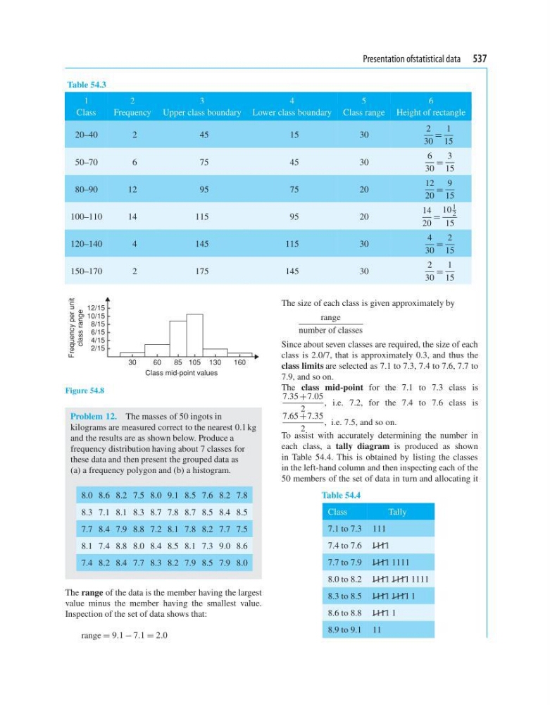
Figure 54.8
Problem 12. The masses of 50 ingots in
kilograms are measured correct to the nearest 0.1 kg
and the results are as shown below. Produce a
frequency distribution having about 7 classes for
these data and then present the grouped data as
(a) a frequency polygon and (b) a histogram.
8.0 8.6 8.2 7.5 8.0 9.1 8.5 7.6 8.2 7.8
8.3 7.1 8.1 8.3 8.7 7.8 8.7 8.5 8.4 8.5
7.7 8.4 7.9 8.8 7.2 8.1 7.8 8.2 7.7 7.5
8.1 7.4 8.8 8.0 8.4 8.5 8.1 7.3 9.0 8.6
7.4 8.2 8.4 7.7 8.3 8.2 7.9 8.5 7.9 8.0
The range of the data is the member having the largest
value minus the member having the smallest value.
Inspection of the set of data shows that:
range = 9.1 − 7.1 = 2.0
The size of each class is given approximately by
range
number of classes
Since about seven classes are required, the size of each
class is 2.0/7, that is approximately 0.3, and thus the
class limits are selected as 7.1 to 7.3, 7.4 to 7.6, 7.7 to
7.9, and so on.
The class mid-point for the 7.1 to 7.3 class is
7.35 +7.05
2
, i.e. 7.2, for the 7.4 to 7.6 class is
7.65 +7.35
2
, i.e. 7.5, and so on.
To assist with accurately determining the number in
each class, a tally diagram is produced as shown
in Table 54.4. This is obtained by listing the classes
in the left-hand column and then inspecting each of the
50 members of the set of data in turn and allocating it
Table 54.4
Class
Tally
7.1 to 7.3 111
7.4 to 7.6 1111
7.7 to 7.9 1111 1111
8.0 to 8.2 1111 1111 1111
8.3 to 8.5 1111 1111 1
8.6 to 8.8 1111 1
8.9 to 9.1 11
Table 54.3
1
2
3
4
5
6
Class
Frequency Upper class boundary Lower class boundary Class range Height of rectangle
20–40
2
45
15
30
2
30
=
1
15
50–70
6
75
45
30
6
30
=
3
15
80–90
12
95
75
20
12
20
=
9
15
100–110
14
115
95
20
14
20
=
10
1
2
15
120–140
4
145
115
30
4
30
=
2
15
150–170
2
175
145
30
2
30
=
1
15
30
4/15
2/15
6/15
Frequency per unit
class range
10/15
8/15
12/15
60
85
Class mid-point values
130
160
105
Figure 54.8
Problem 12. The masses of 50 ingots in
kilograms are measured correct to the nearest 0.1 kg
and the results are as shown below. Produce a
frequency distribution having about 7 classes for
these data and then present the grouped data as
(a) a frequency polygon and (b) a histogram.
8.0 8.6 8.2 7.5 8.0 9.1 8.5 7.6 8.2 7.8
8.3 7.1 8.1 8.3 8.7 7.8 8.7 8.5 8.4 8.5
7.7 8.4 7.9 8.8 7.2 8.1 7.8 8.2 7.7 7.5
8.1 7.4 8.8 8.0 8.4 8.5 8.1 7.3 9.0 8.6
7.4 8.2 8.4 7.7 8.3 8.2 7.9 8.5 7.9 8.0
The range of the data is the member having the largest
value minus the member having the smallest value.
Inspection of the set of data shows that:
range = 9.1 − 7.1 = 2.0
The size of each class is given approximately by
range
number of classes
Since about seven classes are required, the size of each
class is 2.0/7, that is approximately 0.3, and thus the
class limits are selected as 7.1 to 7.3, 7.4 to 7.6, 7.7 to
7.9, and so on.
The class mid-point for the 7.1 to 7.3 class is
7.35 +7.05
2
, i.e. 7.2, for the 7.4 to 7.6 class is
7.65 +7.35
2
, i.e. 7.5, and so on.
To assist with accurately determining the number in
each class, a tally diagram is produced as shown
in Table 54.4. This is obtained by listing the classes
in the left-hand column and then inspecting each of the
50 members of the set of data in turn and allocating it
Table 54.4
Class
Tally
7.1 to 7.3 111
7.4 to 7.6 1111
7.7 to 7.9 1111 1111
8.0 to 8.2 1111 1111 1111
8.3 to 8.5 1111 1111 1
8.6 to 8.8 1111 1
8.9 to 9.1 11