

536 Higher Engineering Mathematics
Table 54.1(a)
Class
Tally
70–72 1
73–75 11
76–78 1111 11
79–81 1111 1111 11
82–84 1111 1111
85–87 1111 1
88–90 111
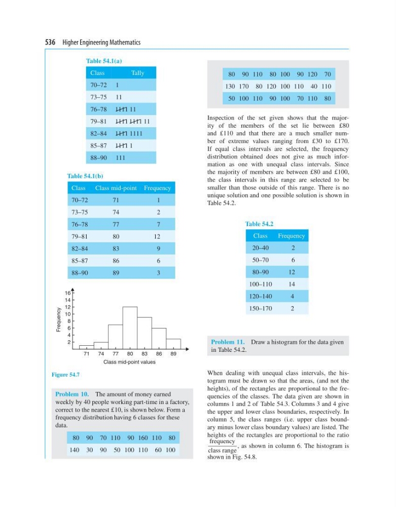
Table 54.1(b)
Class
Class mid-point Frequency
70–72
71
1
73–75
74
2
76–78
77
7
79–81
80
12
82–84
83
9
85–87
86
6
88–90
89
3
71
4
2
6
Frequency
10
8
12
14
16
74
77
80
83
Class mid-point values
89
86
Figure 54.7
Problem 10. The amount of money earned
weekly by 40 people working part-time in a factory,
correct to the nearest £10, is shown below. Form a
frequency distribution having 6 classes for these
data.
80 90 70 110 90 160 110 80
140 30 90 50 100 110 60 100
80 90 110 80 100 90 120 70
130 170 80 120 100 110 40 110
50 100 110 90 100 70 110 80
Inspection of the set given shows that the majority of the members of the set lie between £80
and £110 and that there are a much smaller number of extreme values ranging from £30 to £170.
If equal class intervals are selected, the frequency
distribution obtained does not give as much information as one with unequal class intervals. Since
the majority of members are between £80 and £100,
the class intervals in this range are selected to be
smaller than those outside of this range. There is no
unique solution and one possible solution is shown in
Table 54.2.
Table 54.2
Class
Frequency
20–40
2
50–70
6
80–90
12
100–110
14
120–140
4
150–170
2
Problem 11. Draw a histogram for the data given
in Table 54.2.
When dealing with unequal class intervals, the histogram must be drawn so that the areas, (and not the
heights), of the rectangles are proportional to the frequencies of the classes. The data given are shown in
columns 1 and 2 of Table 54.3. Columns 3 and 4 give
the upper and lower class boundaries, respectively. In
column 5, the class ranges (i.e. upper class boundary minus lower class boundary values) are listed. The
heights of the rectangles are proportional to the ratio
frequency
class range
, as shown in column 6. The histogram is
shown in Fig. 54.8.
Table 54.1(a)
Class
Tally
70–72 1
73–75 11
76–78 1111 11
79–81 1111 1111 11
82–84 1111 1111
85–87 1111 1
88–90 111
Table 54.1(b)
Class
Class mid-point Frequency
70–72
71
1
73–75
74
2
76–78
77
7
79–81
80
12
82–84
83
9
85–87
86
6
88–90
89
3
71
4
2
6
Frequency
10
8
12
14
16
74
77
80
83
Class mid-point values
89
86
Figure 54.7
Problem 10. The amount of money earned
weekly by 40 people working part-time in a factory,
correct to the nearest £10, is shown below. Form a
frequency distribution having 6 classes for these
data.
80 90 70 110 90 160 110 80
140 30 90 50 100 110 60 100
80 90 110 80 100 90 120 70
130 170 80 120 100 110 40 110
50 100 110 90 100 70 110 80
Inspection of the set given shows that the majority of the members of the set lie between £80
and £110 and that there are a much smaller number of extreme values ranging from £30 to £170.
If equal class intervals are selected, the frequency
distribution obtained does not give as much information as one with unequal class intervals. Since
the majority of members are between £80 and £100,
the class intervals in this range are selected to be
smaller than those outside of this range. There is no
unique solution and one possible solution is shown in
Table 54.2.
Table 54.2
Class
Frequency
20–40
2
50–70
6
80–90
12
100–110
14
120–140
4
150–170
2
Problem 11. Draw a histogram for the data given
in Table 54.2.
When dealing with unequal class intervals, the histogram must be drawn so that the areas, (and not the
heights), of the rectangles are proportional to the frequencies of the classes. The data given are shown in
columns 1 and 2 of Table 54.3. Columns 3 and 4 give
the upper and lower class boundaries, respectively. In
column 5, the class ranges (i.e. upper class boundary minus lower class boundary values) are listed. The
heights of the rectangles are proportional to the ratio
frequency
class range
, as shown in column 6. The histogram is
shown in Fig. 54.8.