

An introduction to partial differential equations 521
and B n
cnπ
L
is twice the mean value of
g(x)sin
nπ x
L
between x = 0 and x = L
i.e.
B n =
L
cnπ
2
L
L
0
g(x)sin
nπ x
L
dx
or
B n =
2
cnπ
L
0
g(x)sin
nπ x
L
dx
(9)
Summary of solution of the wave equation
The above may seem complicated; however a practical problem may be solved using the following 8-point
procedure:
1. Identify clearly the initial and boundary
conditions.
2. Assume a solution of the form u = XT and express
the equations in terms of X and T and their
derivatives.
3. Separate the variables by transposing the equation
and equate each side to a constant, say, μ; two
separate equations are obtained, one in x and the
other in t .
4. Let μ =−p 2 to give an oscillatory solution.
5. The two solutions are of the form:
X = A cos px + B sin px
and T = C cos cpt + D sin cpt.
Then u(x, t ) ={A cos px + B sin px}{C cos cpt +
D sin cpt }.
6. Apply the boundary conditions to determine constants A and B.
7. Determine the general solution as an infinite sum.
8. Apply the remaining initial and boundary conditions and determine the coefficients A n and B n
from equations (8) and (9), using Fourier series
techniques.
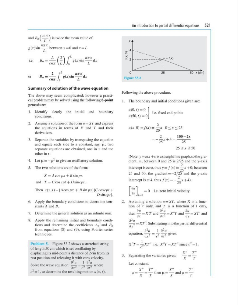
Problem 5. Figure 53.2 shows a stretched string
of length 50 cm which is set oscillating by
displacing its mid-point a distance of 2 cm from its
rest position and releasing it with zero velocity.
Solve the wave equation:
∂ 2 u
∂x 2 =
1
c 2
∂ 2 u
∂t 2 where
c 2 = 1, to determine the resulting motion u(x, t ).
0
2
4
25
50 x (cm)
u(x, 0 )
u 5 f (x )
y
Figure 53.2
Following the above procedure,
1. The boundary and initial conditions given are:
u(0, t ) = 0
u(50, t ) = 0
i.e. fixed end points
u(x, 0) = f (x) =
2
25
x 0 ≤ x ≤ 25
= −
2
25
x + 4 =
100 −2x
25
25 ≤ x ≤ 50
(Note: y = mx + c is a straight line graph, so the gradient, m, between 0 and 25 is 2/25 and the y-axis
intercept is zero, thus y = f (x) =
2
25
x + 0; between
25 and 50, the gradient =−2/25 and the y-axis
intercept is at 4, thus f (x) = −
2
25
x + 4).
∂u
∂t
t =0
= 0 i.e. zero initial velocity.
2. Assuming a solution u = XT , where X is a function of x only, and T is a function of t only,
then
∂u
∂x
= X T and
∂ 2 u
∂x 2 = X T and
∂u
∂ y
= XT and
∂ 2 u
∂ y 2 = XT . Substituting into the partial differential
equation,
∂ 2 u
∂x 2 =
1
c 2
∂ 2 u
∂t 2 gives:
X T =
1
c 2 XT i.e. X T = XT since c 2 = 1.
3. Separating the variables gives:
X
X
=
T
T
Let constant,
μ =
X
X
=
T
T
then μ =
X
X
and μ =
T
T
and B n
cnπ
L
is twice the mean value of
g(x)sin
nπ x
L
between x = 0 and x = L
i.e.
B n =
L
cnπ
2
L
L
0
g(x)sin
nπ x
L
dx
or
B n =
2
cnπ
L
0
g(x)sin
nπ x
L
dx
(9)
Summary of solution of the wave equation
The above may seem complicated; however a practical problem may be solved using the following 8-point
procedure:
1. Identify clearly the initial and boundary
conditions.
2. Assume a solution of the form u = XT and express
the equations in terms of X and T and their
derivatives.
3. Separate the variables by transposing the equation
and equate each side to a constant, say, μ; two
separate equations are obtained, one in x and the
other in t .
4. Let μ =−p 2 to give an oscillatory solution.
5. The two solutions are of the form:
X = A cos px + B sin px
and T = C cos cpt + D sin cpt.
Then u(x, t ) ={A cos px + B sin px}{C cos cpt +
D sin cpt }.
6. Apply the boundary conditions to determine constants A and B.
7. Determine the general solution as an infinite sum.
8. Apply the remaining initial and boundary conditions and determine the coefficients A n and B n
from equations (8) and (9), using Fourier series
techniques.
Problem 5. Figure 53.2 shows a stretched string
of length 50 cm which is set oscillating by
displacing its mid-point a distance of 2 cm from its
rest position and releasing it with zero velocity.
Solve the wave equation:
∂ 2 u
∂x 2 =
1
c 2
∂ 2 u
∂t 2 where
c 2 = 1, to determine the resulting motion u(x, t ).
0
2
4
25
50 x (cm)
u(x, 0 )
u 5 f (x )
y
Figure 53.2
Following the above procedure,
1. The boundary and initial conditions given are:
u(0, t ) = 0
u(50, t ) = 0
i.e. fixed end points
u(x, 0) = f (x) =
2
25
x 0 ≤ x ≤ 25
= −
2
25
x + 4 =
100 −2x
25
25 ≤ x ≤ 50
(Note: y = mx + c is a straight line graph, so the gradient, m, between 0 and 25 is 2/25 and the y-axis
intercept is zero, thus y = f (x) =
2
25
x + 0; between
25 and 50, the gradient =−2/25 and the y-axis
intercept is at 4, thus f (x) = −
2
25
x + 4).
∂u
∂t
t =0
= 0 i.e. zero initial velocity.
2. Assuming a solution u = XT , where X is a function of x only, and T is a function of t only,
then
∂u
∂x
= X T and
∂ 2 u
∂x 2 = X T and
∂u
∂ y
= XT and
∂ 2 u
∂ y 2 = XT . Substituting into the partial differential
equation,
∂ 2 u
∂x 2 =
1
c 2
∂ 2 u
∂t 2 gives:
X T =
1
c 2 XT i.e. X T = XT since c 2 = 1.
3. Separating the variables gives:
X
X
=
T
T
Let constant,
μ =
X
X
=
T
T
then μ =
X
X
and μ =
T
T