Numerical methods for first order differential equations 473
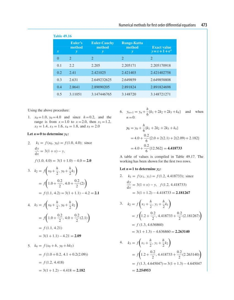
Table 49.16
Euler’s
Euler-Cauchy
Runge-Kutta
method
method
method
Exact value
x
y
y
y
y = x +1 + e x
0
2
2
2
2
0.1
2.2
2.205
2.205171
2.205170918
0.2
2.41
2.421025
2.421403
2.421402758
0.3
2.631
2.649232625
2.649859
2.649858808
0.4
2.8641
2.89090205
2.891824
2.891824698
0.5
3.11051
3.147446765
3.148720
3.148721271
Using the above procedure:
1. x 0 = 1.0, y 0 = 4.0 and since h = 0.2, and the
range is from x = 1.0 to x = 2.0, then x 1 = 1.2,
x 2 = 1.4, x 3 = 1.6, x 4 = 1.8, and x 5 = 2.0
Let n = 0 to determine y 1 :
2. k 1 = f (x 0 , y 0 ) = f (1.0, 4.0); since
d y
dx
= 3(1 + x) − y,
f (1.0, 4.0) = 3(1 + 1.0) − 4.0 = 2.0
3. k 2 = f
x 0 +
h
2
, y 0 +
h
2
k 1
= f
1.0 +
0.2
2
, 4.0 +
0.2
2
(2)
= f (1.1, 4.2) = 3(1 + 1.1) − 4.2 = 2.1
4. k 3 = f
x 0 +
h
2
, y 0 +
h
2
k 2
= f
1.0 +
0.2
2
, 4.0 +
0.2
2
(2.1)
= f (1.1, 4.21)
= 3(1 + 1.1) − 4.21 = 2.09
5. k 4 = f (x 0 + h, y 0 + hk 3 )
= f (1.0 + 0.2, 4.1 + 0.2(2.09))
= f (1.2, 4.418)
= 3(1 + 1.2) − 4.418 = 2.182
6. y n+1 = y n +
h
6
{k 1 + 2k 2 + 2k 3 + k 4 } and when
n = 0:
y 1 = y 0 +
h
6
{k 1 + 2k 2 + 2k 3 + k 4 }
= 4.0 +
0.2
6
{2.0 + 2(2.1) + 2(2.09) + 2.182}
= 4.0 +
0.2
6
{12.562} = 4.418733
A table of values is compiled in Table 49.17. The
working has been shown for the first two rows.
Let n = 1 to determine y 2 :
2. k 1 = f (x 1 , y 1 ) = f (1.2, 4.418733); since
d y
dx
= 3(1 + x) − y, f (1.2, 4.418733)
= 3(1 + 1.2) − 4.418733 = 2.181267
3. k 2 = f
x 1 +
h
2
, y 1 +
h
2
k 1
= f
1.2 +
0.2
2
, 4.418733 +
0.2
2
(2.181267)
= f (1.3, 4.636860)
= 3(1 + 1.3) − 4.636860 = 2.263140
4. k 3 = f
x 1 +
h
2
, y 1 +
h
2
k 2
= f
1.2 +
0.2
2
, 4.418733 +
0.2
2
(2.263140)
= f (1.3, 4.645047) = 3(1 + 1.3) − 4.645047
= 2.254953