

474 Higher Engineering Mathematics
Table 49.17
n
x n
k 1
k 2
k 3
k 4
y n
0
1.0
4.0
1
1.2
2.0
2.1
2.09
2.182
4.418733
2
1.4
2.181267
2.263140
2.254953
2.330276
4.870324
3
1.6
2.329676
2.396708
2.390005
2.451675
5.348817
4
1.8
2.451183
2.506065
2.500577
2.551068
5.849335
5
2.0
2.550665
2.595599
2.591105
2.632444
6.367886
5. k 4 = f (x 1 + h, y 1 + hk 3 )
= f (1.2 + 0.2, 4.418733 + 0.2(2.254953))
= f (1.4, 4.869724) = 3(1 + 1.4) − 4.869724
= 2.330276
6. y n+1 = y n +
h
6
{k 1 + 2k 2 + 2k 3 + k 4 } and when
n =1:
y 2 = y 1 +
h
6
{k 1 + 2k 2 + 2k 3 + k 4 }
= 4.418733 +
0.2
6
{2.181267 + 2(2.263140)
+ 2(2.254953) + 2.330276}
= 4.418733 +
0.2
6
{13.547729} = 4.870324
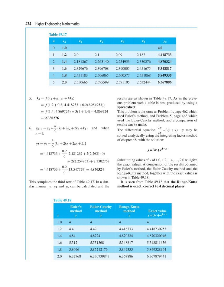
This completes the third row of Table 49.17. In a similar manner y 3 , y 4 and y 5 can be calculated and the
results are as shown in Table 49.17. As in the previous problem such a table is best produced by using a
spreadsheet.
This problem is the same as Problem 1, page 462 which
used Euler’s method, and Problem 5, page 468 which
used the Euler-Cauchy method, and a comparison of
results can be made.
The differential equation
d y
dx
= 3(1 + x) − y may be
solved analytically using the integrating factor method
of chapter 48, with the solution:
y = 3x +e
1−x
Substituting values of x of 1.0, 1.2, 1.4, ..., 2.0 will give
the exact values. A comparison of the results obtained
by Euler’s method, the Euler-Cauchy method and the
Runga-Kutta method, together with the exact values is
shown in Table 49.18.
It is seen from Table 49.18 that the Runge-Kutta
method is exact, correct to 4 decimal places.
Table 49.18
Euler’s
Euler-Cauchy
Runge-Kutta
method
method
method
Exact value
x
y
y
y
y = 3x + e 1−x
1.0
4
4
4
4
1.2
4.4
4.42
4.418733
4.418730753
1.4
4.84
4.8724
4.870324
4.870320046
1.6
5.312
5.351368
5.348817
5.348811636
1.8
5.8096
5.85212176
5.849335
5.849328964
2.0
6.32768
6.370739847
6.367886
6.367879441
Table 49.17
n
x n
k 1
k 2
k 3
k 4
y n
0
1.0
4.0
1
1.2
2.0
2.1
2.09
2.182
4.418733
2
1.4
2.181267
2.263140
2.254953
2.330276
4.870324
3
1.6
2.329676
2.396708
2.390005
2.451675
5.348817
4
1.8
2.451183
2.506065
2.500577
2.551068
5.849335
5
2.0
2.550665
2.595599
2.591105
2.632444
6.367886
5. k 4 = f (x 1 + h, y 1 + hk 3 )
= f (1.2 + 0.2, 4.418733 + 0.2(2.254953))
= f (1.4, 4.869724) = 3(1 + 1.4) − 4.869724
= 2.330276
6. y n+1 = y n +
h
6
{k 1 + 2k 2 + 2k 3 + k 4 } and when
n =1:
y 2 = y 1 +
h
6
{k 1 + 2k 2 + 2k 3 + k 4 }
= 4.418733 +
0.2
6
{2.181267 + 2(2.263140)
+ 2(2.254953) + 2.330276}
= 4.418733 +
0.2
6
{13.547729} = 4.870324
This completes the third row of Table 49.17. In a similar manner y 3 , y 4 and y 5 can be calculated and the
results are as shown in Table 49.17. As in the previous problem such a table is best produced by using a
spreadsheet.
This problem is the same as Problem 1, page 462 which
used Euler’s method, and Problem 5, page 468 which
used the Euler-Cauchy method, and a comparison of
results can be made.
The differential equation
d y
dx
= 3(1 + x) − y may be
solved analytically using the integrating factor method
of chapter 48, with the solution:
y = 3x +e
1−x
Substituting values of x of 1.0, 1.2, 1.4, ..., 2.0 will give
the exact values. A comparison of the results obtained
by Euler’s method, the Euler-Cauchy method and the
Runga-Kutta method, together with the exact values is
shown in Table 49.18.
It is seen from Table 49.18 that the Runge-Kutta
method is exact, correct to 4 decimal places.
Table 49.18
Euler’s
Euler-Cauchy
Runge-Kutta
method
method
method
Exact value
x
y
y
y
y = 3x + e 1−x
1.0
4
4
4
4
1.2
4.4
4.42
4.418733
4.418730753
1.4
4.84
4.8724
4.870324
4.870320046
1.6
5.312
5.351368
5.348817
5.348811636
1.8
5.8096
5.85212176
5.849335
5.849328964
2.0
6.32768
6.370739847
6.367886
6.367879441