

472 Higher Engineering Mathematics
Table 49.15
n
x n
k 1
k 2
k 3
k 4
y n
0
0
2
1
0.1
2.0
2.05
2.0525
2.10525
2.205171
2
0.2
2.105171
2.160430
2.163193
2.221490
2.421403
3
0.3
2.221403
2.282473
2.285527
2.349956
2.649859
4
0.4
2.349859
2.417339
2.420726
2.491932
2.891824
5
0.5
2.491824
2.566415
2.570145
2.648838
3.148720
Let n =1 to determine y 2 :
2.
k 1 = f (x 1 , y 1 ) = f (0.1, 2.205171); since
d y
dx
= y − x, f (0.1, 2.205171)
= 2.205171 − 0.1 = 2.105171
3. k 2 = f
x 1 +
h
2
, y 1 +
h
2
k 1
= f
0.1 +
0.1
2
, 2.205171 +
0.1
2
(2.105171)
= f (0.15, 2.31042955)
= 2.31042955 − 0.15 = 2.160430
4. k 3 = f
x 1 +
h
2
, y 1 +
h
2
k 2
= f
0.1 +
0.1
2
, 2.205171 +
0.1
2
(2.160430)
= f (0.15, 2.3131925) = 2.3131925 − 0.15
= 2.163193
5. k 4 = f (x 1 + h, y 1 + hk 3 )
= f (0.1 + 0.1, 2.205171 + 0.1(2.163193))
= f (0.2, 2.421490)
= 2.421490 − 0.2 = 2.221490
6. y n+1 = y n +
h
6
{k 1 + 2k 2 + 2k 3 + k 4 }
and when n = 1:
y 2 = y 1 +
h
6
{k 1 + 2k 2 + 2k 3 + k 4 }
= 2.205171+
0.1
6
{2.105171+2(2.160430)
+ 2(2.163193) + 2.221490}
= 2.205171 +
0.1
6
{12.973907} = 2.421403
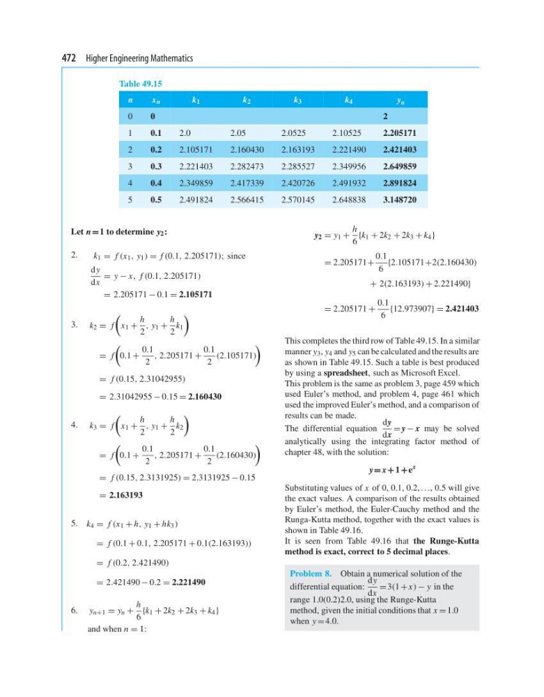
This completes the third row of Table 49.15. In a similar
manner y 3 , y 4 and y 5 can be calculated and the results are
as shown in Table 49.15. Such a table is best produced
by using a spreadsheet, such as Microsoft Excel.
This problem is the same as problem 3, page 459 which
used Euler’s method, and problem 4, page 461 which
used the improved Euler’s method, and a comparison of
results can be made.
The differential equation
dy
dx
= y − x may be solved
analytically using the integrating factor method of
chapter 48, with the solution:
y = x + 1 +e
x
Substituting values of x of 0, 0.1, 0.2, ..., 0.5 will give
the exact values. A comparison of the results obtained
by Euler’s method, the Euler-Cauchy method and the
Runga-Kutta method, together with the exact values is
shown in Table 49.16.
It is seen from Table 49.16 that the Runge-Kutta
method is exact, correct to 5 decimal places.
Problem 8. Obtain a numerical solution of the
differential equation:
d y
dx
= 3(1 + x) − y in the
range 1.0(0.2)2.0, using the Runge-Kutta
method, given the initial conditions that x = 1.0
when y = 4.0.
Table 49.15
n
x n
k 1
k 2
k 3
k 4
y n
0
0
2
1
0.1
2.0
2.05
2.0525
2.10525
2.205171
2
0.2
2.105171
2.160430
2.163193
2.221490
2.421403
3
0.3
2.221403
2.282473
2.285527
2.349956
2.649859
4
0.4
2.349859
2.417339
2.420726
2.491932
2.891824
5
0.5
2.491824
2.566415
2.570145
2.648838
3.148720
Let n =1 to determine y 2 :
2.
k 1 = f (x 1 , y 1 ) = f (0.1, 2.205171); since
d y
dx
= y − x, f (0.1, 2.205171)
= 2.205171 − 0.1 = 2.105171
3. k 2 = f
x 1 +
h
2
, y 1 +
h
2
k 1
= f
0.1 +
0.1
2
, 2.205171 +
0.1
2
(2.105171)
= f (0.15, 2.31042955)
= 2.31042955 − 0.15 = 2.160430
4. k 3 = f
x 1 +
h
2
, y 1 +
h
2
k 2
= f
0.1 +
0.1
2
, 2.205171 +
0.1
2
(2.160430)
= f (0.15, 2.3131925) = 2.3131925 − 0.15
= 2.163193
5. k 4 = f (x 1 + h, y 1 + hk 3 )
= f (0.1 + 0.1, 2.205171 + 0.1(2.163193))
= f (0.2, 2.421490)
= 2.421490 − 0.2 = 2.221490
6. y n+1 = y n +
h
6
{k 1 + 2k 2 + 2k 3 + k 4 }
and when n = 1:
y 2 = y 1 +
h
6
{k 1 + 2k 2 + 2k 3 + k 4 }
= 2.205171+
0.1
6
{2.105171+2(2.160430)
+ 2(2.163193) + 2.221490}
= 2.205171 +
0.1
6
{12.973907} = 2.421403
This completes the third row of Table 49.15. In a similar
manner y 3 , y 4 and y 5 can be calculated and the results are
as shown in Table 49.15. Such a table is best produced
by using a spreadsheet, such as Microsoft Excel.
This problem is the same as problem 3, page 459 which
used Euler’s method, and problem 4, page 461 which
used the improved Euler’s method, and a comparison of
results can be made.
The differential equation
dy
dx
= y − x may be solved
analytically using the integrating factor method of
chapter 48, with the solution:
y = x + 1 +e
x
Substituting values of x of 0, 0.1, 0.2, ..., 0.5 will give
the exact values. A comparison of the results obtained
by Euler’s method, the Euler-Cauchy method and the
Runga-Kutta method, together with the exact values is
shown in Table 49.16.
It is seen from Table 49.16 that the Runge-Kutta
method is exact, correct to 5 decimal places.
Problem 8. Obtain a numerical solution of the
differential equation:
d y
dx
= 3(1 + x) − y in the
range 1.0(0.2)2.0, using the Runge-Kutta
method, given the initial conditions that x = 1.0
when y = 4.0.