

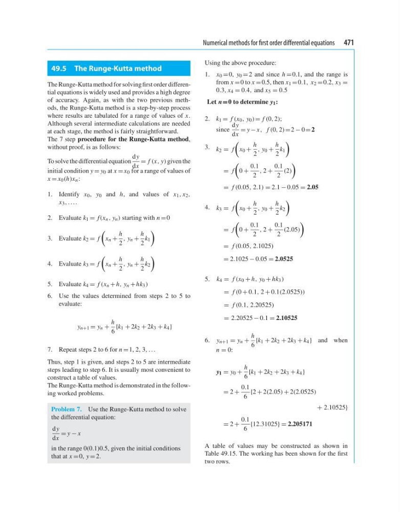
Numerical methods for first order differential equations 471
49.5 The Runge-Kutta method
The Runge-Kutta method for solving first order differential equations is widely used and provides a high degree
of accuracy. Again, as with the two previous methods, the Runge-Kutta method is a step-by-step process
where results are tabulated for a range of values of x.
Although several intermediate calculations are needed
at each stage, the method is fairly straightforward.
The 7 step procedure for the Runge-Kutta method,
without proof, is as follows:
To solve the differential equation
d y
dx
= f (x, y) given the
initial condition y = y 0 at x = x 0 for a range of values of
x = x 0 (h)x n :
1. Identify x 0 , y 0 and h, and values of x 1 , x 2 ,
x 3 , ....
2. Evaluate k 1 = f(x n , y n ) starting with n =0
3. Evaluate k 2 = f
x n +
h
2
, y n +
h
2
k 1
4. Evaluate k 3 = f
x n +
h
2
, y n +
h
2
k 2
5. Evaluate k 4 = f (x n + h, y n + hk 3 )
6. Use the values determined from steps 2 to 5 to
evaluate:
y n+1 = y n +
h
6
{k 1 + 2k 2 + 2k 3 + k 4 }
7. Repeat steps 2 to 6 for n = 1, 2, 3, ...
Thus, step 1 is given, and steps 2 to 5 are intermediate
steps leading to step 6. It is usually most convenient to
construct a table of values.
The Runge-Kutta method is demonstrated in the following worked problems.
Problem 7. Use the Runge-Kutta method to solve
the differential equation:
d y
dx
= y − x
in the range 0(0.1)0.5, given the initial conditions
that at x = 0, y = 2.
Using the above procedure:
1. x 0 = 0, y 0 = 2 and since h = 0.1, and the range is
from x = 0 to x = 0.5, then x 1 = 0.1, x 2 = 0.2, x 3 =
0.3, x 4 = 0.4, and x 5 = 0.5
Let n =0 to determine y 1 :
2. k 1 = f (x 0 , y 0 ) = f (0, 2);
since
d y
dx
= y − x, f (0, 2) =2 − 0 = 2
3. k 2 = f
x 0 +
h
2
, y 0 +
h
2
k 1
= f
0 +
0.1
2
, 2 +
0.1
2
(2)
= f (0.05, 2.1) = 2.1 − 0.05 = 2.05
4. k 3 = f
x 0 +
h
2
, y 0 +
h
2
k 2
= f
0 +
0.1
2
, 2 +
0.1
2
(2.05)
= f (0.05, 2.1025)
= 2.1025 − 0.05 = 2.0525
5. k 4 = f (x 0 + h, y 0 + hk 3 )
= f (0 + 0.1, 2 + 0.1(2.0525))
= f (0.1, 2.20525)
= 2.20525 − 0.1 = 2.10525
6. y n+1 = y n +
h
6
{k 1 + 2k 2 + 2k 3 + k 4 } and when
n = 0:
y 1 = y 0 +
h
6
{k 1 + 2k 2 + 2k 3 + k 4 }
= 2 +
0.1
6
{2 + 2(2.05) + 2(2.0525)
+ 2.10525}
= 2 +
0.1
6
{12.31025} = 2.205171
A table of values may be constructed as shown in
Table 49.15. The working has been shown for the first
two rows.
49.5 The Runge-Kutta method
The Runge-Kutta method for solving first order differential equations is widely used and provides a high degree
of accuracy. Again, as with the two previous methods, the Runge-Kutta method is a step-by-step process
where results are tabulated for a range of values of x.
Although several intermediate calculations are needed
at each stage, the method is fairly straightforward.
The 7 step procedure for the Runge-Kutta method,
without proof, is as follows:
To solve the differential equation
d y
dx
= f (x, y) given the
initial condition y = y 0 at x = x 0 for a range of values of
x = x 0 (h)x n :
1. Identify x 0 , y 0 and h, and values of x 1 , x 2 ,
x 3 , ....
2. Evaluate k 1 = f(x n , y n ) starting with n =0
3. Evaluate k 2 = f
x n +
h
2
, y n +
h
2
k 1
4. Evaluate k 3 = f
x n +
h
2
, y n +
h
2
k 2
5. Evaluate k 4 = f (x n + h, y n + hk 3 )
6. Use the values determined from steps 2 to 5 to
evaluate:
y n+1 = y n +
h
6
{k 1 + 2k 2 + 2k 3 + k 4 }
7. Repeat steps 2 to 6 for n = 1, 2, 3, ...
Thus, step 1 is given, and steps 2 to 5 are intermediate
steps leading to step 6. It is usually most convenient to
construct a table of values.
The Runge-Kutta method is demonstrated in the following worked problems.
Problem 7. Use the Runge-Kutta method to solve
the differential equation:
d y
dx
= y − x
in the range 0(0.1)0.5, given the initial conditions
that at x = 0, y = 2.
Using the above procedure:
1. x 0 = 0, y 0 = 2 and since h = 0.1, and the range is
from x = 0 to x = 0.5, then x 1 = 0.1, x 2 = 0.2, x 3 =
0.3, x 4 = 0.4, and x 5 = 0.5
Let n =0 to determine y 1 :
2. k 1 = f (x 0 , y 0 ) = f (0, 2);
since
d y
dx
= y − x, f (0, 2) =2 − 0 = 2
3. k 2 = f
x 0 +
h
2
, y 0 +
h
2
k 1
= f
0 +
0.1
2
, 2 +
0.1
2
(2)
= f (0.05, 2.1) = 2.1 − 0.05 = 2.05
4. k 3 = f
x 0 +
h
2
, y 0 +
h
2
k 2
= f
0 +
0.1
2
, 2 +
0.1
2
(2.05)
= f (0.05, 2.1025)
= 2.1025 − 0.05 = 2.0525
5. k 4 = f (x 0 + h, y 0 + hk 3 )
= f (0 + 0.1, 2 + 0.1(2.0525))
= f (0.1, 2.20525)
= 2.20525 − 0.1 = 2.10525
6. y n+1 = y n +
h
6
{k 1 + 2k 2 + 2k 3 + k 4 } and when
n = 0:
y 1 = y 0 +
h
6
{k 1 + 2k 2 + 2k 3 + k 4 }
= 2 +
0.1
6
{2 + 2(2.05) + 2(2.0525)
+ 2.10525}
= 2 +
0.1
6
{12.31025} = 2.205171
A table of values may be constructed as shown in
Table 49.15. The working has been shown for the first
two rows.