

Numerical methods for first order differential equations 465
For line 4, where x 0 = 0.3:
y 1 = y 0 + h(y
) 0
= 2.41 + (0.1)(2.21) = 2.631
and ( y
) 0 = y 0 − x 0
= 2.631 − 0.3 = 2.331
For line 5, where x 0 = 0.4:
y 1 = y 0 + h(y
) 0
= 2.631 + (0.1)(2.331) = 2.8641
and ( y
) 0 = y 0 − x 0
= 2.8641 − 0.4 = 2.4641
For line 6, where x 0 = 0.5:
y 1 = y 0 + h(y
) 0
= 2.8641 + (0.1)(2.4641) = 3.11051
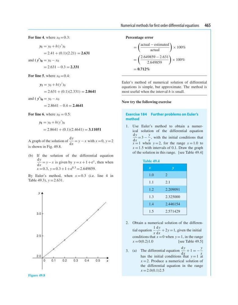
A graph of the solution of
d y
dx
= y − x with x = 0, y = 2
is shown in Fig. 49.8.
(b) If the solution of the differential equation
d y
dx
= y − x is given by y = x + 1 +e x , then when
x = 0.3, y = 0.3 + 1 +e 0.3 = 2.649859.
By Euler’s method, when x = 0.3 (i.e. line 4 in
Table 49.3), y = 2.631.
y
x
3.0
2.5
2.0
0
0.1
0.2
0.3
0.4
0.5
Figure 49.8
Percentage error
=
actual − estimated
actual
× 100%
=
2.649859 − 2.631
2.649859
× 100%
= 0.712%
Euler’s method of numerical solution of differential
equations is simple, but approximate. The method is
most useful when the interval h is small.
Now try the following exercise
Exercise 184 Further problems on Euler’s
method
1. Use Euler’s method to obtain a numerical solution of the differential equation
d y
dx
= 3 −
y
x
, with the initial conditions that
x = 1 when y = 2, for the range x = 1.0 to
x = 1.5 with intervals of 0.1. Draw the graph
of the solution in this range. [see Table 49.4]
Table 49.4
x
y
1.0
2
1.1
2.1
1.2
2.209091
1.3
2.325000
1.4
2.446154
1.5
2.571429
2. Obtain a numerical solution of the differential equation
1
x
d y
dx
+ 2y = 1, given the initial
conditions that x = 0 when y = 1, in the range
x = 0(0.2)1.0
[see Table 49.5]
3. (a) The differential equation
d y
dx
+ 1 = −
y
x
has the initial conditions that y = 1 at
x = 2. Produce a numerical solution of
the differential equation in the range
x = 2.0(0.1)2.5
For line 4, where x 0 = 0.3:
y 1 = y 0 + h(y
) 0
= 2.41 + (0.1)(2.21) = 2.631
and ( y
) 0 = y 0 − x 0
= 2.631 − 0.3 = 2.331
For line 5, where x 0 = 0.4:
y 1 = y 0 + h(y
) 0
= 2.631 + (0.1)(2.331) = 2.8641
and ( y
) 0 = y 0 − x 0
= 2.8641 − 0.4 = 2.4641
For line 6, where x 0 = 0.5:
y 1 = y 0 + h(y
) 0
= 2.8641 + (0.1)(2.4641) = 3.11051
A graph of the solution of
d y
dx
= y − x with x = 0, y = 2
is shown in Fig. 49.8.
(b) If the solution of the differential equation
d y
dx
= y − x is given by y = x + 1 +e x , then when
x = 0.3, y = 0.3 + 1 +e 0.3 = 2.649859.
By Euler’s method, when x = 0.3 (i.e. line 4 in
Table 49.3), y = 2.631.
y
x
3.0
2.5
2.0
0
0.1
0.2
0.3
0.4
0.5
Figure 49.8
Percentage error
=
actual − estimated
actual
× 100%
=
2.649859 − 2.631
2.649859
× 100%
= 0.712%
Euler’s method of numerical solution of differential
equations is simple, but approximate. The method is
most useful when the interval h is small.
Now try the following exercise
Exercise 184 Further problems on Euler’s
method
1. Use Euler’s method to obtain a numerical solution of the differential equation
d y
dx
= 3 −
y
x
, with the initial conditions that
x = 1 when y = 2, for the range x = 1.0 to
x = 1.5 with intervals of 0.1. Draw the graph
of the solution in this range. [see Table 49.4]
Table 49.4
x
y
1.0
2
1.1
2.1
1.2
2.209091
1.3
2.325000
1.4
2.446154
1.5
2.571429
2. Obtain a numerical solution of the differential equation
1
x
d y
dx
+ 2y = 1, given the initial
conditions that x = 0 when y = 1, in the range
x = 0(0.2)1.0
[see Table 49.5]
3. (a) The differential equation
d y
dx
+ 1 = −
y
x
has the initial conditions that y = 1 at
x = 2. Produce a numerical solution of
the differential equation in the range
x = 2.0(0.1)2.5