

466 Higher Engineering Mathematics
Table 49.5
x
y
0
1
0.2
1
0.4
0.96
0.6
0.8864
0.8
0.793664
1.0
0.699692
(b) If the solution of the differential equation by an analytical method is given
by y =
4
x
−
x
2
, determine the percentage
error at x = 2.2
[(a) see Table 49.6 (b) 1.206%]
Table 49.6
x
y
2.0
1
2.1
0.85
2.2
0.709524
2.3
0.577273
2.4
0.452174
2.5
0.333334
4. Use Euler’s method to obtain a numerical solution of the differential equation
d y
dx
= x −
2y
x
,
given the initial conditions that y = 1 when
x = 2, in the range x = 2.0(0.2)3.0.
If the solution of the differential equation is
given by y =
x 2
4
, determine the percentage
error by using Euler’s method when x = 2.8
[see Table 49.7, 1.596%]
Table 49.7
x
y
2.0
1
2.2
1.2
2.4
1.421818
2.6
1.664849
2.8
1.928718
3.0
2.213187
49.4 An improved Euler method
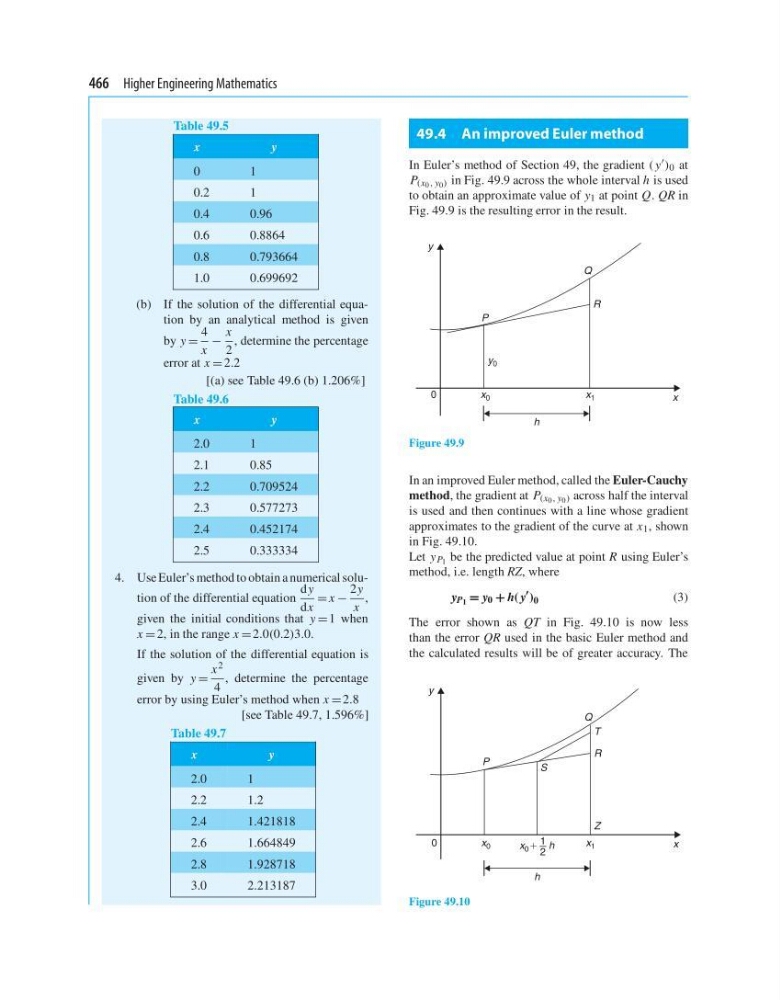
In Euler’s method of Section 49, the gradient ( y ) 0 at
P (x 0 , y 0 ) in Fig. 49.9 across the whole interval h is used
to obtain an approximate value of y 1 at point Q. QR in
Fig. 49.9 is the resulting error in the result.
y
P
x 0
x 1
x
Q
R
y 0
0
h
Figure 49.9
In an improved Euler method, called the Euler-Cauchy
method, the gradient at P (x 0 , y 0 ) across half the interval
is used and then continues with a line whose gradient
approximates to the gradient of the curve at x 1 , shown
in Fig. 49.10.
Let y P 1 be the predicted value at point R using Euler’s
method, i.e. length RZ, where
y P 1 = y 0 + h( y
) 0
(3)
The error shown as QT in Fig. 49.10 is now less
than the error QR used in the basic Euler method and
the calculated results will be of greater accuracy. The
y
P
S
x 0
x 1
x
Q
R
Z
T
0
h
x 0
h
1 1
2
Figure 49.10
Table 49.5
x
y
0
1
0.2
1
0.4
0.96
0.6
0.8864
0.8
0.793664
1.0
0.699692
(b) If the solution of the differential equation by an analytical method is given
by y =
4
x
−
x
2
, determine the percentage
error at x = 2.2
[(a) see Table 49.6 (b) 1.206%]
Table 49.6
x
y
2.0
1
2.1
0.85
2.2
0.709524
2.3
0.577273
2.4
0.452174
2.5
0.333334
4. Use Euler’s method to obtain a numerical solution of the differential equation
d y
dx
= x −
2y
x
,
given the initial conditions that y = 1 when
x = 2, in the range x = 2.0(0.2)3.0.
If the solution of the differential equation is
given by y =
x 2
4
, determine the percentage
error by using Euler’s method when x = 2.8
[see Table 49.7, 1.596%]
Table 49.7
x
y
2.0
1
2.2
1.2
2.4
1.421818
2.6
1.664849
2.8
1.928718
3.0
2.213187
49.4 An improved Euler method
In Euler’s method of Section 49, the gradient ( y ) 0 at
P (x 0 , y 0 ) in Fig. 49.9 across the whole interval h is used
to obtain an approximate value of y 1 at point Q. QR in
Fig. 49.9 is the resulting error in the result.
y
P
x 0
x 1
x
Q
R
y 0
0
h
Figure 49.9
In an improved Euler method, called the Euler-Cauchy
method, the gradient at P (x 0 , y 0 ) across half the interval
is used and then continues with a line whose gradient
approximates to the gradient of the curve at x 1 , shown
in Fig. 49.10.
Let y P 1 be the predicted value at point R using Euler’s
method, i.e. length RZ, where
y P 1 = y 0 + h( y
) 0
(3)
The error shown as QT in Fig. 49.10 is now less
than the error QR used in the basic Euler method and
the calculated results will be of greater accuracy. The
y
P
S
x 0
x 1
x
Q
R
Z
T
0
h
x 0
h
1 1
2
Figure 49.10