

464 Higher Engineering Mathematics
For line 2, where x 0 = 0.2 and h = 0.2:
y 1 = y 0 + h(y
), from equation (2)
= 1 + (0.2)(−1) = 0.8
and ( y
) 0 = 2x 0 − y 0 = 2(0.2) − 0.8 = −0.4
For line 3, where x 0 = 0.4:
y 1 = y 0 + h(y
) 0
= 0.8 + (0.2)(−0.4) = 0.72
and ( y
) 0 = 2x 0 − y 0 = 2(0.4) − 0.72 = 0.08
For line 4, where x 0 = 0.6:
y 1 = y 0 + h(y
) 0
= 0.72 + (0.2)(0.08) = 0.736
and ( y
) 0 = 2x 0 − y 0 = 2(0.6) − 0.736 = 0.464
For line 5, where x 0 = 0.8:
y 1 = y 0 + h(y
) 0
= 0.736 + (0.2)(0.464) = 0.8288
and ( y
) 0 = 2x 0 − y 0 = 2(0.8) − 0.8288 = 0.7712
For line 6, where x 0 = 1.0:
y 1 = y 0 + h(y
) 0
= 0.8288 + (0.2)(0.7712) = 0.98304
As the range is 0 to 1.0, ( y ) 0 in line 6 is not needed.
y
x
1.0
0.5
0
0.2
0.4
0.6
0.8
1.0
Figure 49.7
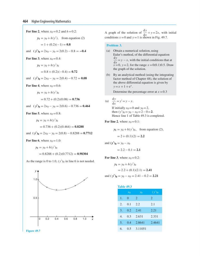
A graph of the solution of
d y
dx
+ y = 2x, with initial
conditions x = 0 and y = 1 is shown in Fig. 49.7.
Problem 3.
(a) Obtain a numerical solution, using
Euler’s method, of the differential equation
d y
dx
= y − x, with the initial conditions that at
x = 0, y = 2, for the range x = 0(0.1)0.5. Draw
the graph of the solution.
(b) By an analytical method (using the integrating
factor method of Chapter 48), the solution of
the above differential equation is given by
y = x + 1 + e x .
Determine the percentage error at x = 0.3
(a)
d y
dx
= y = y − x.
If initially x 0 = 0 and y 0 = 2,
then (y ) 0 = y 0 − x 0 = 2 − 0 =2.
Hence line 1 of Table 49.3 is completed.
For line 2, where x 0 = 0.1:
y 1 = y 0 + h(y
) 0 , from equation (2),
= 2 + (0.1)(2) = 2.2
and (y
) 0 = y 0 − x 0
= 2.2 − 0.1 = 2.1
For line 3, where x 0 = 0.2:
y 1 = y 0 + h(y
) 0
= 2.2 + (0.1)(2.1) = 2.41
and ( y
) 0 = y 0 − x 0 = 2.41 − 0.2 = 2.21
Table 49.3
x 0
y 0
( y ) 0
1. 0
2
2
2. 0.1 2.2
2.1
3. 0.2 2.41
2.21
4. 0.3 2.631
2.331
5. 0.4 2.8641
2.4641
6. 0.5 3.11051
For line 2, where x 0 = 0.2 and h = 0.2:
y 1 = y 0 + h(y
), from equation (2)
= 1 + (0.2)(−1) = 0.8
and ( y
) 0 = 2x 0 − y 0 = 2(0.2) − 0.8 = −0.4
For line 3, where x 0 = 0.4:
y 1 = y 0 + h(y
) 0
= 0.8 + (0.2)(−0.4) = 0.72
and ( y
) 0 = 2x 0 − y 0 = 2(0.4) − 0.72 = 0.08
For line 4, where x 0 = 0.6:
y 1 = y 0 + h(y
) 0
= 0.72 + (0.2)(0.08) = 0.736
and ( y
) 0 = 2x 0 − y 0 = 2(0.6) − 0.736 = 0.464
For line 5, where x 0 = 0.8:
y 1 = y 0 + h(y
) 0
= 0.736 + (0.2)(0.464) = 0.8288
and ( y
) 0 = 2x 0 − y 0 = 2(0.8) − 0.8288 = 0.7712
For line 6, where x 0 = 1.0:
y 1 = y 0 + h(y
) 0
= 0.8288 + (0.2)(0.7712) = 0.98304
As the range is 0 to 1.0, ( y ) 0 in line 6 is not needed.
y
x
1.0
0.5
0
0.2
0.4
0.6
0.8
1.0
Figure 49.7
A graph of the solution of
d y
dx
+ y = 2x, with initial
conditions x = 0 and y = 1 is shown in Fig. 49.7.
Problem 3.
(a) Obtain a numerical solution, using
Euler’s method, of the differential equation
d y
dx
= y − x, with the initial conditions that at
x = 0, y = 2, for the range x = 0(0.1)0.5. Draw
the graph of the solution.
(b) By an analytical method (using the integrating
factor method of Chapter 48), the solution of
the above differential equation is given by
y = x + 1 + e x .
Determine the percentage error at x = 0.3
(a)
d y
dx
= y = y − x.
If initially x 0 = 0 and y 0 = 2,
then (y ) 0 = y 0 − x 0 = 2 − 0 =2.
Hence line 1 of Table 49.3 is completed.
For line 2, where x 0 = 0.1:
y 1 = y 0 + h(y
) 0 , from equation (2),
= 2 + (0.1)(2) = 2.2
and (y
) 0 = y 0 − x 0
= 2.2 − 0.1 = 2.1
For line 3, where x 0 = 0.2:
y 1 = y 0 + h(y
) 0
= 2.2 + (0.1)(2.1) = 2.41
and ( y
) 0 = y 0 − x 0 = 2.41 − 0.2 = 2.21
Table 49.3
x 0
y 0
( y ) 0
1. 0
2
2
2. 0.1 2.2
2.1
3. 0.2 2.41
2.21
4. 0.3 2.631
2.331
5. 0.4 2.8641
2.4641
6. 0.5 3.11051