

Numerical methods for first order differential equations 463
This step by step Euler’s method can be continued
and it is easiest to list the results in a table, as shown
in Table 49.1. The results for lines 1 to 3 have been
produced above.
Table 49.1
x 0
y 0
(y ) 0
1.
1
4
2
2.
1.2
4.4
2.2
3.
1.4
4.84
2.36
4.
1.6
5.312
2.488
5.
1.8
5.8096
2.5904
6.
2.0
6.32768
For line 4, where x 0 = 1.6:
y 1 = y 0 + h( y
) 0
= 4.84 + (0.2)(2.36) = 5.312
and ( y
) 0 = 3(1 + 1.6) − 5.312 = 2.488
For line 5, where x 0 = 1.8:
y 1 = y 0 + h(y
) 0
= 5.312 + (0.2)(2.488) = 5.8096
and ( y
) 0 = 3(1 + 1.8) − 5.8096 = 2.5904
For line 6, where x 0 = 2.0:
y 1 = y 0 + h(y
) 0
= 5.8096 + (0.2)(2.5904)
= 6.32768
(As the range is 1.0 to 2.0 there is no need to calculate
(y ) 0 in line 6). The particular solution is given by the
value of y against x.
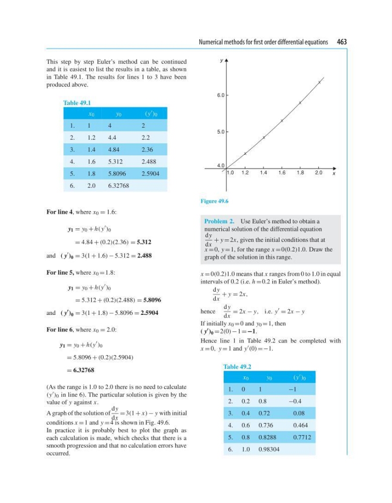
A graph of the solution of
d y
dx
= 3(1 + x) − y with initial
conditions x = 1 and y = 4 is shown in Fig. 49.6.
In practice it is probably best to plot the graph as
each calculation is made, which checks that there is a
smooth progression and that no calculation errors have
occurred.
y
x
6.0
5.0
4.0
1.0
1.2
1.4
1.6
1.8
2.0
Figure 49.6
Problem 2. Use Euler’s method to obtain a
numerical solution of the differential equation
d y
dx
+ y = 2x, given the initial conditions that at
x = 0, y = 1, for the range x = 0(0.2)1.0. Draw the
graph of the solution in this range.
x = 0(0.2)1.0 means that x ranges from 0 to 1.0 in equal
intervals of 0.2 (i.e. h =0.2 in Euler’s method).
d y
dx
+ y = 2x,
hence
d y
dx
= 2x − y, i.e. y
= 2x − y
If initially x 0 = 0 and y 0 = 1, then
( y ) 0 = 2(0) − 1 = −1.
Hence line 1 in Table 49.2 can be completed with
x = 0, y = 1 and y (0) =−1.
Table 49.2
x 0
y 0
(y ) 0
1. 0
1
−1
2. 0.2 0.8
−0.4
3. 0.4 0.72
0.08
4. 0.6 0.736
0.464
5. 0.8 0.8288
0.7712
6. 1.0 0.98304
This step by step Euler’s method can be continued
and it is easiest to list the results in a table, as shown
in Table 49.1. The results for lines 1 to 3 have been
produced above.
Table 49.1
x 0
y 0
(y ) 0
1.
1
4
2
2.
1.2
4.4
2.2
3.
1.4
4.84
2.36
4.
1.6
5.312
2.488
5.
1.8
5.8096
2.5904
6.
2.0
6.32768
For line 4, where x 0 = 1.6:
y 1 = y 0 + h( y
) 0
= 4.84 + (0.2)(2.36) = 5.312
and ( y
) 0 = 3(1 + 1.6) − 5.312 = 2.488
For line 5, where x 0 = 1.8:
y 1 = y 0 + h(y
) 0
= 5.312 + (0.2)(2.488) = 5.8096
and ( y
) 0 = 3(1 + 1.8) − 5.8096 = 2.5904
For line 6, where x 0 = 2.0:
y 1 = y 0 + h(y
) 0
= 5.8096 + (0.2)(2.5904)
= 6.32768
(As the range is 1.0 to 2.0 there is no need to calculate
(y ) 0 in line 6). The particular solution is given by the
value of y against x.
A graph of the solution of
d y
dx
= 3(1 + x) − y with initial
conditions x = 1 and y = 4 is shown in Fig. 49.6.
In practice it is probably best to plot the graph as
each calculation is made, which checks that there is a
smooth progression and that no calculation errors have
occurred.
y
x
6.0
5.0
4.0
1.0
1.2
1.4
1.6
1.8
2.0
Figure 49.6
Problem 2. Use Euler’s method to obtain a
numerical solution of the differential equation
d y
dx
+ y = 2x, given the initial conditions that at
x = 0, y = 1, for the range x = 0(0.2)1.0. Draw the
graph of the solution in this range.
x = 0(0.2)1.0 means that x ranges from 0 to 1.0 in equal
intervals of 0.2 (i.e. h =0.2 in Euler’s method).
d y
dx
+ y = 2x,
hence
d y
dx
= 2x − y, i.e. y
= 2x − y
If initially x 0 = 0 and y 0 = 1, then
( y ) 0 = 2(0) − 1 = −1.
Hence line 1 in Table 49.2 can be completed with
x = 0, y = 1 and y (0) =−1.
Table 49.2
x 0
y 0
(y ) 0
1. 0
1
−1
2. 0.2 0.8
−0.4
3. 0.4 0.72
0.08
4. 0.6 0.736
0.464
5. 0.8 0.8288
0.7712
6. 1.0 0.98304