

462 Higher Engineering Mathematics
which is a statement called Taylor’s series.
If h is the interval between two new ordinates y 0 and
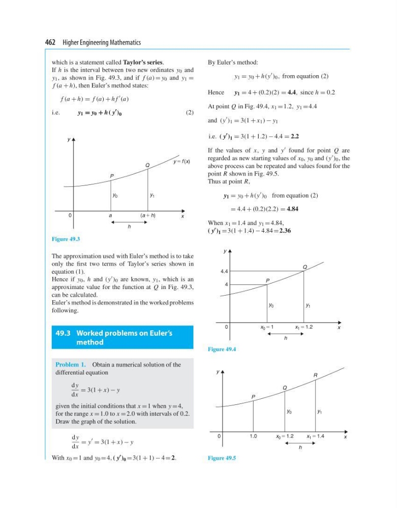
y 1 , as shown in Fig. 49.3, and if f (a) = y 0 and y 1 =
f (a + h), then Euler’s method states:
f (a + h) = f (a) + h f
(a)
i.e.
y 1 = y 0 + h ( y
) 0
(2)
y
y 5 f (x)
P
h
a
x
Q
y 0
y 1
(a 1 h)
0
Figure 49.3
The approximation used with Euler’s method is to take
only the first two terms of Taylor’s series shown in
equation (1).
Hence if y 0 , h and (y ) 0 are known, y 1 , which is an
approximate value for the function at Q in Fig. 49.3,
can be calculated.
Euler’s method is demonstrated in the worked problems
following.
49.3 Worked problems on Euler’s
method
Problem 1. Obtain a numerical solution of the
differential equation
d y
dx
= 3(1 + x) − y
given the initial conditions that x = 1 when y = 4,
for the range x = 1.0 to x = 2.0 with intervals of 0.2.
Draw the graph of the solution.
d y
dx
= y
= 3(1 + x) − y
With x 0 = 1 and y 0 = 4, ( y ) 0 = 3(1 + 1) − 4 = 2.
By Euler’s method:
y 1 = y 0 + h(y
) 0 , from equation (2)
Hence
y 1 = 4 + (0.2)(2) = 4.4, since h = 0.2
At point Q in Fig. 49.4, x 1 = 1.2, y 1 = 4.4
and (y
) 1 = 3(1 + x 1 ) − y 1
i.e. ( y
) 1 = 3(1 + 1.2) − 4.4 = 2.2
If the values of x, y and y found for point Q are
regarded as new starting values of x 0 , y 0 and (y ) 0 , the
above process can be repeated and values found for the
point R shown in Fig. 49.5.
Thus at point R,
y 1 = y 0 + h(y
) 0 from equation (2)
= 4.4 + (0.2)(2.2) = 4.84
When x 1 = 1.4 and y 1 = 4.84,
( y ) 1 = 3(1 + 1.4) − 4.84 = 2.36
y
P
h
x
Q
y 0
x 0 5 1
x 1 5 1.2
y 1
0
4
4.4
Figure 49.4
y
P
h
x
Q
R
y 0
x 0 5 1.2
x 1 5 1.4
y 1
0
1.0
Figure 49.5
which is a statement called Taylor’s series.
If h is the interval between two new ordinates y 0 and
y 1 , as shown in Fig. 49.3, and if f (a) = y 0 and y 1 =
f (a + h), then Euler’s method states:
f (a + h) = f (a) + h f
(a)
i.e.
y 1 = y 0 + h ( y
) 0
(2)
y
y 5 f (x)
P
h
a
x
Q
y 0
y 1
(a 1 h)
0
Figure 49.3
The approximation used with Euler’s method is to take
only the first two terms of Taylor’s series shown in
equation (1).
Hence if y 0 , h and (y ) 0 are known, y 1 , which is an
approximate value for the function at Q in Fig. 49.3,
can be calculated.
Euler’s method is demonstrated in the worked problems
following.
49.3 Worked problems on Euler’s
method
Problem 1. Obtain a numerical solution of the
differential equation
d y
dx
= 3(1 + x) − y
given the initial conditions that x = 1 when y = 4,
for the range x = 1.0 to x = 2.0 with intervals of 0.2.
Draw the graph of the solution.
d y
dx
= y
= 3(1 + x) − y
With x 0 = 1 and y 0 = 4, ( y ) 0 = 3(1 + 1) − 4 = 2.
By Euler’s method:
y 1 = y 0 + h(y
) 0 , from equation (2)
Hence
y 1 = 4 + (0.2)(2) = 4.4, since h = 0.2
At point Q in Fig. 49.4, x 1 = 1.2, y 1 = 4.4
and (y
) 1 = 3(1 + x 1 ) − y 1
i.e. ( y
) 1 = 3(1 + 1.2) − 4.4 = 2.2
If the values of x, y and y found for point Q are
regarded as new starting values of x 0 , y 0 and (y ) 0 , the
above process can be repeated and values found for the
point R shown in Fig. 49.5.
Thus at point R,
y 1 = y 0 + h(y
) 0 from equation (2)
= 4.4 + (0.2)(2.2) = 4.84
When x 1 = 1.4 and y 1 = 4.84,
( y ) 1 = 3(1 + 1.4) − 4.84 = 2.36
y
P
h
x
Q
y 0
x 0 5 1
x 1 5 1.2
y 1
0
4
4.4
Figure 49.4
y
P
h
x
Q
R
y 0
x 0 5 1.2
x 1 5 1.4
y 1
0
1.0
Figure 49.5