

Chapter 49
Numerical methods for
first order differential
equations
49.1 Introduction
Not all first order differential equations may be solved
by separating the variables (as in Chapter 46) or by the
integrating factor method (as in Chapter 48). A number
of other analytical methods of solving differential equations exist. However the differential equations that can
be solved by such analytical methods is fairly restricted.
Where a differential equation and known boundary
conditions are given, an approximate solution may be
obtained by applying a numerical method. There are
a number of such numerical methods available and the
simplest of these is called Euler’s method.
49.2 Euler’s method
From Chapter 8, Maclaurin’s series may be stated as:
f (x) = f (0) + x f
(0) +
x 2
2!
f
(0) + · · ·
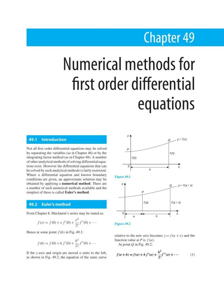
Hence at some point f (h) in Fig. 49.1:
f (h) = f (0) + h f
(0) +
h 2
2!
f
(0) + · · ·
If the y-axis and origin are moved a units to the left,
as shown in Fig. 49.2, the equation of the same curve
y
y 5 f (x )
P
h
x
Q
f (0)
f (h)
0
Figure 49.1
y
y 5 f (a 1 x)
P
h
a
x
Q
f (a)
f (a 1 x)
0
Figure 49.2
relative to the new axis becomes y = f (a + x) and the
function value at P is f (a).
At point Q in Fig. 49.2:
f (a + h) = f (a) + h f
(a) +
h 2
2!
f
(a) + · · ·
(1)
Numerical methods for
first order differential
equations
49.1 Introduction
Not all first order differential equations may be solved
by separating the variables (as in Chapter 46) or by the
integrating factor method (as in Chapter 48). A number
of other analytical methods of solving differential equations exist. However the differential equations that can
be solved by such analytical methods is fairly restricted.
Where a differential equation and known boundary
conditions are given, an approximate solution may be
obtained by applying a numerical method. There are
a number of such numerical methods available and the
simplest of these is called Euler’s method.
49.2 Euler’s method
From Chapter 8, Maclaurin’s series may be stated as:
f (x) = f (0) + x f
(0) +
x 2
2!
f
(0) + · · ·
Hence at some point f (h) in Fig. 49.1:
f (h) = f (0) + h f
(0) +
h 2
2!
f
(0) + · · ·
If the y-axis and origin are moved a units to the left,
as shown in Fig. 49.2, the equation of the same curve
y
y 5 f (x )
P
h
x
Q
f (0)
f (h)
0
Figure 49.1
y
y 5 f (a 1 x)
P
h
a
x
Q
f (a)
f (a 1 x)
0
Figure 49.2
relative to the new axis becomes y = f (a + x) and the
function value at P is f (a).
At point Q in Fig. 49.2:
f (a + h) = f (a) + h f
(a) +
h 2
2!
f
(a) + · · ·
(1)