

Methods of differentiation 289
Substituting (x + δx) for x gives
f (x + δx) = (x + δx) 2 = x 2 + 2xδx + δx 2 , hence
f
(x) = limit
δx→0
(x
2
+ 2xδx + δx
2
) − (x
2
)
δx
= limit
δx→0
(2xδx + δx 2 )
δx
= limit
δx→0
[2x + δx]
As δx → 0, [2x + δx] →[2x + 0]. Thus f (x) = 2x, i.e.
the differential coefficient of x 2 is 2x. At x = 2, the
gradient of the curve, f (x) = 2(2) = 4.
Differentiation from first principles can be a lengthy
process and it would not be convenient to go through this
procedure every time we want to differentiate a function.
In reality we do not have to because a set of general
rules have evolved from the above procedure, which we
consider in the following section.
27.4 Differentiation of common
functions
From differentiation by first principles of a number of
examples such as in Problem 1 above, a general rule
for differentiating y = ax
n emerges, where a and n are
constants.
The rule is: if y = ax
n then
dy
dx
= anx
n−1
(or, if f (x)= ax n then f (x)= anx n−1 ) and is true for all
real values of a and n.
For example, if y = 4x 3 then a = 4 and n =3, and
d y
dx
= anx
n−1
= (4)(3)x
3−1
= 12x
2
If y = ax n and n =0 then y = ax 0 and
d y
dx
= (a)(0)x
0−1
= 0,
i.e. the differential coefficient of a constant is zero.
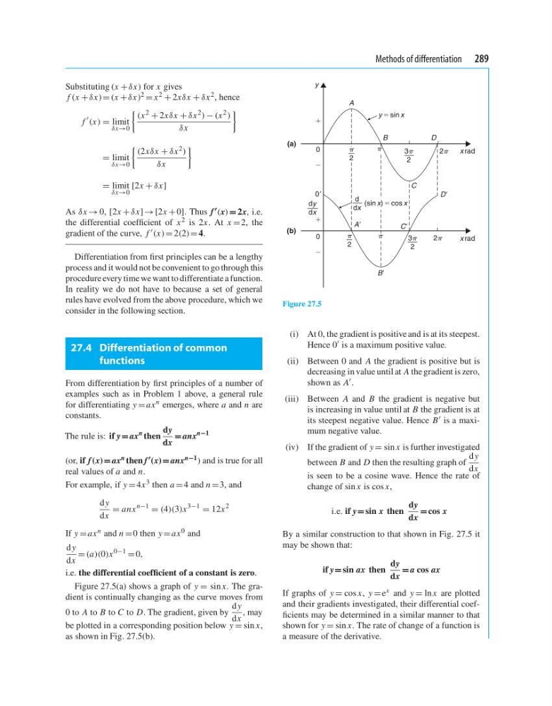
Figure 27.5(a) shows a graph of y = sin x. The gradient is continually changing as the curve moves from
0 to A to B to C to D. The gradient, given by
d y
dx
, may
be plotted in a corresponding position below y = sin x,
as shown in Fig. 27.5(b).
y
0
(a)
(b)
0
y ϭ sin x
x rad
x rad
ϩ
Ϫ
Ϫ
A
AЈ
0Ј
CЈ
BЈ
DЈ
B
D
C
2
d
dx
ϩ
dy
dx
2
2
3
2
3
2
(sin x) ϭ cos x
2
Figure 27.5
(i) At 0, the gradient is positive and is at its steepest.
Hence 0 is a maximum positive value.
(ii) Between 0 and A the gradient is positive but is
decreasing in value until at A the gradient is zero,
shown as A .
(iii) Between A and B the gradient is negative but
is increasing in value until at B the gradient is at
its steepest negative value. Hence B is a maximum negative value.
(iv) If the gradient of y = sin x is further investigated
between B and D then the resulting graph of
d y
dx
is seen to be a cosine wave. Hence the rate of
change of sin x is cos x,
i.e. if y = sin x then
dy
dx
= cos x
By a similar construction to that shown in Fig. 27.5 it
may be shown that:
if y = sin ax then
dy
dx
= a cos ax
If graphs of y = cos x, y = e x and y = ln x are plotted
and their gradients investigated, their differential coefficients may be determined in a similar manner to that
shown for y = sin x. The rate of change of a function is
a measure of the derivative.
Substituting (x + δx) for x gives
f (x + δx) = (x + δx) 2 = x 2 + 2xδx + δx 2 , hence
f
(x) = limit
δx→0
(x
2
+ 2xδx + δx
2
) − (x
2
)
δx
= limit
δx→0
(2xδx + δx 2 )
δx
= limit
δx→0
[2x + δx]
As δx → 0, [2x + δx] →[2x + 0]. Thus f (x) = 2x, i.e.
the differential coefficient of x 2 is 2x. At x = 2, the
gradient of the curve, f (x) = 2(2) = 4.
Differentiation from first principles can be a lengthy
process and it would not be convenient to go through this
procedure every time we want to differentiate a function.
In reality we do not have to because a set of general
rules have evolved from the above procedure, which we
consider in the following section.
27.4 Differentiation of common
functions
From differentiation by first principles of a number of
examples such as in Problem 1 above, a general rule
for differentiating y = ax
n emerges, where a and n are
constants.
The rule is: if y = ax
n then
dy
dx
= anx
n−1
(or, if f (x)= ax n then f (x)= anx n−1 ) and is true for all
real values of a and n.
For example, if y = 4x 3 then a = 4 and n =3, and
d y
dx
= anx
n−1
= (4)(3)x
3−1
= 12x
2
If y = ax n and n =0 then y = ax 0 and
d y
dx
= (a)(0)x
0−1
= 0,
i.e. the differential coefficient of a constant is zero.
Figure 27.5(a) shows a graph of y = sin x. The gradient is continually changing as the curve moves from
0 to A to B to C to D. The gradient, given by
d y
dx
, may
be plotted in a corresponding position below y = sin x,
as shown in Fig. 27.5(b).
y
0
(a)
(b)
0
y ϭ sin x
x rad
x rad
ϩ
Ϫ
Ϫ
A
AЈ
0Ј
CЈ
BЈ
DЈ
B
D
C
2
d
dx
ϩ
dy
dx
2
2
3
2
3
2
(sin x) ϭ cos x
2
Figure 27.5
(i) At 0, the gradient is positive and is at its steepest.
Hence 0 is a maximum positive value.
(ii) Between 0 and A the gradient is positive but is
decreasing in value until at A the gradient is zero,
shown as A .
(iii) Between A and B the gradient is negative but
is increasing in value until at B the gradient is at
its steepest negative value. Hence B is a maximum negative value.
(iv) If the gradient of y = sin x is further investigated
between B and D then the resulting graph of
d y
dx
is seen to be a cosine wave. Hence the rate of
change of sin x is cos x,
i.e. if y = sin x then
dy
dx
= cos x
By a similar construction to that shown in Fig. 27.5 it
may be shown that:
if y = sin ax then
dy
dx
= a cos ax
If graphs of y = cos x, y = e x and y = ln x are plotted
and their gradients investigated, their differential coefficients may be determined in a similar manner to that
shown for y = sin x. The rate of change of a function is
a measure of the derivative.