

288 Higher Engineering Mathematics
0
1
1.5
2
3
2
4
6
8
10
f(x)
x
A
D
C
B f(x) 5 x
2
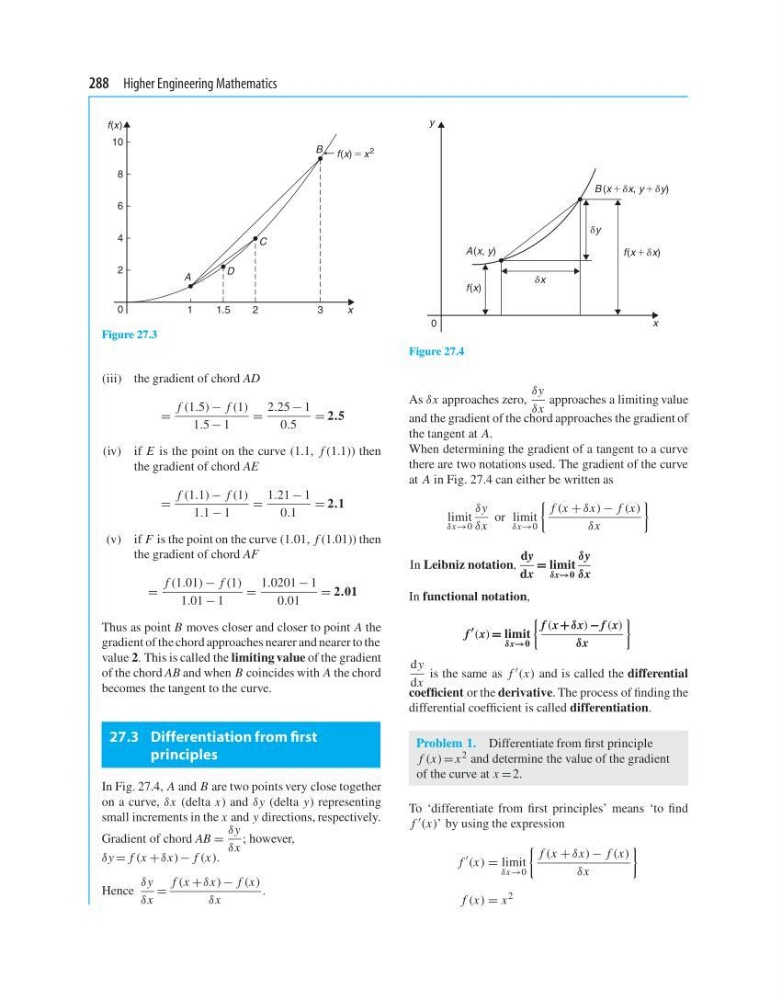
Figure 27.3
(iii) the gradient of chord AD
=
f (1.5) − f (1)
1.5 − 1
=
2.25 − 1
0.5
= 2.5
(iv) if E is the point on the curve (1.1, f (1.1)) then
the gradient of chord AE
=
f (1.1) − f (1)
1.1 − 1
=
1.21 − 1
0.1
= 2.1
(v) if F is the point on the curve (1.01, f (1.01)) then
the gradient of chord AF
=
f (1.01) − f (1)
1.01 − 1
=
1.0201 − 1
0.01
= 2.01
Thus as point B moves closer and closer to point A the
gradient of the chord approaches nearer and nearer to the
value 2. This is called the limiting value of the gradient
of the chord AB and when B coincides with A the chord
becomes the tangent to the curve.
27.3 Differentiation from first
principles
In Fig. 27.4, A and B are two points very close together
on a curve, δx (delta x) and δy (delta y) representing
small increments in the x and y directions, respectively.
Gradient of chord AB =
δy
δx
; however,
δy = f (x + δx) − f (x).
Hence
δy
δx
=
f (x + δx) − f (x)
δx
.
0
y
f(x)
f(x 1 ␦x)
␦y
␦x
x
A(x, y)
B (x 1 ␦x, y 1 ␦y)
Figure 27.4
As δx approaches zero,
δy
δx
approaches a limiting value
and the gradient of the chord approaches the gradient of
the tangent at A.
When determining the gradient of a tangent to a curve
there are two notations used. The gradient of the curve
at A in Fig. 27.4 can either be written as
limit
δx→0
δy
δx
or limit
δx→0
f (x + δx) − f (x)
δx
In Leibniz notation,
dy
dx
= limit
δx→0
δy
δx
In functional notation,
f
(x) = limit
δx→0
f (x +δx) − f (x)
δx
d y
dx
is the same as f (x) and is called the differential
coefficient or the derivative. The process of finding the
differential coefficient is called differentiation.
Problem 1. Differentiate from first principle
f (x) = x 2 and determine the value of the gradient
of the curve at x = 2.
To ‘differentiate from first principles’ means ‘to find
f (x)’ by using the expression
f
(x) = limit
δx→0
f (x + δx) − f (x)
δx
f (x) = x
2
0
1
1.5
2
3
2
4
6
8
10
f(x)
x
A
D
C
B f(x) 5 x
2
Figure 27.3
(iii) the gradient of chord AD
=
f (1.5) − f (1)
1.5 − 1
=
2.25 − 1
0.5
= 2.5
(iv) if E is the point on the curve (1.1, f (1.1)) then
the gradient of chord AE
=
f (1.1) − f (1)
1.1 − 1
=
1.21 − 1
0.1
= 2.1
(v) if F is the point on the curve (1.01, f (1.01)) then
the gradient of chord AF
=
f (1.01) − f (1)
1.01 − 1
=
1.0201 − 1
0.01
= 2.01
Thus as point B moves closer and closer to point A the
gradient of the chord approaches nearer and nearer to the
value 2. This is called the limiting value of the gradient
of the chord AB and when B coincides with A the chord
becomes the tangent to the curve.
27.3 Differentiation from first
principles
In Fig. 27.4, A and B are two points very close together
on a curve, δx (delta x) and δy (delta y) representing
small increments in the x and y directions, respectively.
Gradient of chord AB =
δy
δx
; however,
δy = f (x + δx) − f (x).
Hence
δy
δx
=
f (x + δx) − f (x)
δx
.
0
y
f(x)
f(x 1 ␦x)
␦y
␦x
x
A(x, y)
B (x 1 ␦x, y 1 ␦y)
Figure 27.4
As δx approaches zero,
δy
δx
approaches a limiting value
and the gradient of the chord approaches the gradient of
the tangent at A.
When determining the gradient of a tangent to a curve
there are two notations used. The gradient of the curve
at A in Fig. 27.4 can either be written as
limit
δx→0
δy
δx
or limit
δx→0
f (x + δx) − f (x)
δx
In Leibniz notation,
dy
dx
= limit
δx→0
δy
δx
In functional notation,
f
(x) = limit
δx→0
f (x +δx) − f (x)
δx
d y
dx
is the same as f (x) and is called the differential
coefficient or the derivative. The process of finding the
differential coefficient is called differentiation.
Problem 1. Differentiate from first principle
f (x) = x 2 and determine the value of the gradient
of the curve at x = 2.
To ‘differentiate from first principles’ means ‘to find
f (x)’ by using the expression
f
(x) = limit
δx→0
f (x + δx) − f (x)
δx
f (x) = x
2