

184 Higher Engineering Mathematics
and graphs of y = ln x and y =−ln x are shown in
Fig. 18.19(b).
Problem 1. Sketch the following graphs, showing
relevant points:
(a) y = (x − 4)
2
(b) y = x
3
− 8
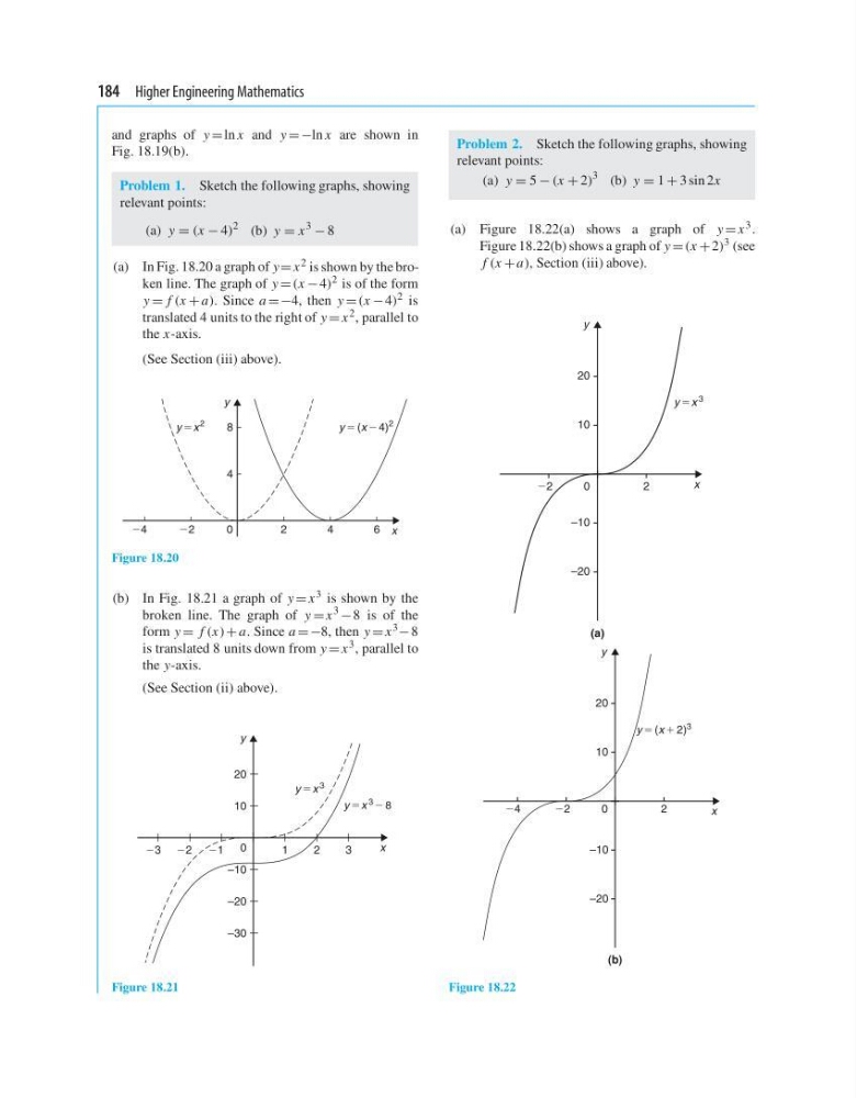
(a) In Fig. 18.20 a graph of y = x 2 is shown by the broken line. The graph of y = (x − 4) 2 is of the form
y = f (x + a). Since a =−4, then y = (x − 4) 2 is
translated 4 units to the right of y = x 2 , parallel to
the x-axis.
(See Section (iii) above).
y ϭx
2
y ϭ (x Ϫ 4)
2
4
Ϫ2
Ϫ4
0
8
2
4
6
y
x
Figure 18.20
(b) In Fig. 18.21 a graph of y = x 3 is shown by the
broken line. The graph of y = x
3
− 8 is of the
form y = f (x) + a. Since a =−8, then y = x 3 − 8
is translated 8 units down from y = x 3 , parallel to
the y-axis.
(See Section (ii) above).
20
10
–10
–20
–30
0
Ϫ1
1
2
3
Ϫ2
Ϫ3
y ϭx 3
y ϭx 3 Ϫ 8
y
x
Figure 18.21
Problem 2. Sketch the following graphs, showing
relevant points:
(a) y = 5 − (x + 2)
3
(b) y = 1 + 3 sin 2x
(a) Figure 18.22(a) shows a graph of y = x 3 .
Figure 18.22(b) shows a graph of y = (x + 2) 3 (see
f (x + a), Section (iii) above).
10
20
y ϭx
3
(a)
–10
–20
0
2
Ϫ2
x
y
24
10
20
y 5 (x 1 2)
3
(b)
–10
–20
0
2
22
x
y
Figure 18.22
and graphs of y = ln x and y =−ln x are shown in
Fig. 18.19(b).
Problem 1. Sketch the following graphs, showing
relevant points:
(a) y = (x − 4)
2
(b) y = x
3
− 8
(a) In Fig. 18.20 a graph of y = x 2 is shown by the broken line. The graph of y = (x − 4) 2 is of the form
y = f (x + a). Since a =−4, then y = (x − 4) 2 is
translated 4 units to the right of y = x 2 , parallel to
the x-axis.
(See Section (iii) above).
y ϭx
2
y ϭ (x Ϫ 4)
2
4
Ϫ2
Ϫ4
0
8
2
4
6
y
x
Figure 18.20
(b) In Fig. 18.21 a graph of y = x 3 is shown by the
broken line. The graph of y = x
3
− 8 is of the
form y = f (x) + a. Since a =−8, then y = x 3 − 8
is translated 8 units down from y = x 3 , parallel to
the y-axis.
(See Section (ii) above).
20
10
–10
–20
–30
0
Ϫ1
1
2
3
Ϫ2
Ϫ3
y ϭx 3
y ϭx 3 Ϫ 8
y
x
Figure 18.21
Problem 2. Sketch the following graphs, showing
relevant points:
(a) y = 5 − (x + 2)
3
(b) y = 1 + 3 sin 2x
(a) Figure 18.22(a) shows a graph of y = x 3 .
Figure 18.22(b) shows a graph of y = (x + 2) 3 (see
f (x + a), Section (iii) above).
10
20
y ϭx
3
(a)
–10
–20
0
2
Ϫ2
x
y
24
10
20
y 5 (x 1 2)
3
(b)
–10
–20
0
2
22
x
y
Figure 18.22