

182 Higher Engineering Mathematics
(b)
0
2
2
1
3
2
3
y ϭ cos ϩ 2
y ϭ cos
y ϭx
y ϭ x ϩ 3
6
4
2
0
2
4
(a)
6
x
y
(c)
0
Ϫ1
1
2
2
4
6
8
Ϫ2
x
y ϭ x
2 ϩ 3
y ϭ x 2
y
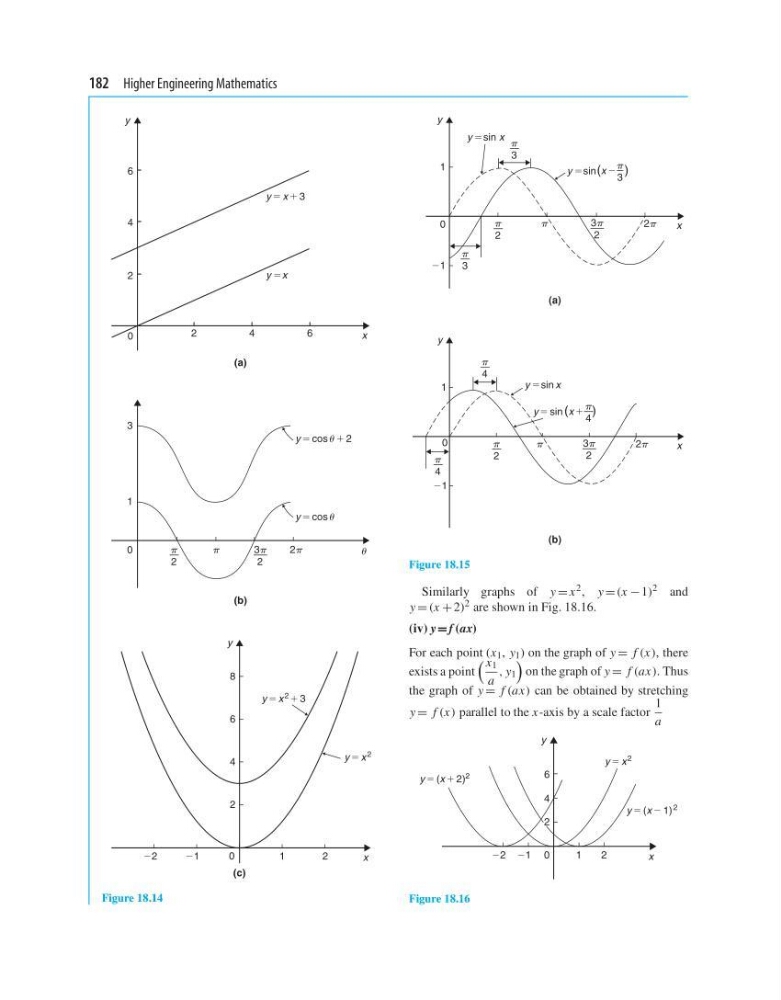
Figure 18.14
0
(a)
(b)
1
1
21
21
0
(x 2 )
y 5sin x
y 5sin x
y 5sin
(x 1 )
y 5 sin
2
2
4
4
3
3
4
3
2
3
2
3
2
2
y
x
x
y
Figure 18.15
Similarly graphs of y = x 2 , y = (x − 1) 2 and
y = (x + 2) 2 are shown in Fig. 18.16.
(iv) y = f (ax)
For each point (x 1 , y 1 ) on the graph of y = f (x), there
exists a point
x 1
a
, y 1
on the graph of y = f (ax). Thus
the graph of y = f (ax) can be obtained by stretching
y = f (x) parallel to the x-axis by a scale factor
1
a
6
4
2
21
1
0
2
22
y 5 (x 1 2) 2
y 5 (x 2 1)
2
y 5 x 2
x
y
Figure 18.16
(b)
0
2
2
1
3
2
3
y ϭ cos ϩ 2
y ϭ cos
y ϭx
y ϭ x ϩ 3
6
4
2
0
2
4
(a)
6
x
y
(c)
0
Ϫ1
1
2
2
4
6
8
Ϫ2
x
y ϭ x
2 ϩ 3
y ϭ x 2
y
Figure 18.14
0
(a)
(b)
1
1
21
21
0
(x 2 )
y 5sin x
y 5sin x
y 5sin
(x 1 )
y 5 sin
2
2
4
4
3
3
4
3
2
3
2
3
2
2
y
x
x
y
Figure 18.15
Similarly graphs of y = x 2 , y = (x − 1) 2 and
y = (x + 2) 2 are shown in Fig. 18.16.
(iv) y = f (ax)
For each point (x 1 , y 1 ) on the graph of y = f (x), there
exists a point
x 1
a
, y 1
on the graph of y = f (ax). Thus
the graph of y = f (ax) can be obtained by stretching
y = f (x) parallel to the x-axis by a scale factor
1
a
6
4
2
21
1
0
2
22
y 5 (x 1 2) 2
y 5 (x 2 1)
2
y 5 x 2
x
y
Figure 18.16