

Functions and their curves 181
0
1
y 5e x
y
x
Figure 18.11
O
a
a
r 5a sin
Figure 18.12
18.2 Simple transformations
From the graph of y = f (x) it is possible to deduce the graphs of other functions which are transformations of y = f (x). For example, knowing the graph
of y = f (x), can help us draw the graphs of y = a f (x),
y = f (x) + a, y = f (x + a), y = f (ax), y =− f (x) and
y = f (−x).
(i) y = af (x)
For each point (x 1 , y 1 ) on the graph of y = f (x) there
exists a point (x 1 , ay 1 ) on the graph of y = a f (x).
Thus the graph of y = a f (x) can be obtained by
stretching y = f (x) parallel to the y-axis by a scale
factor ‘a’.
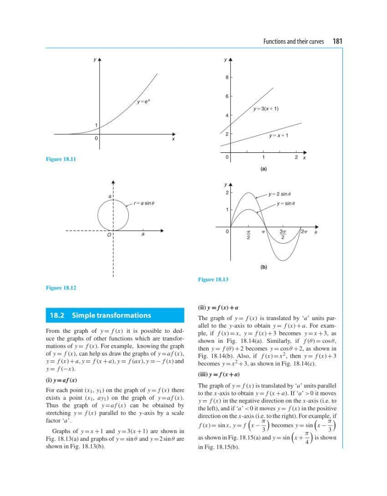
Graphs of y = x + 1 and y = 3(x + 1) are shown in
Fig. 18.13(a) and graphs of y = sin θ and y = 2 sin θ are
shown in Fig. 18.13(b).
0
2
3
2
2
1
2
(b)
(a)
8
6
4
2
0
1
2
y
y
y 5 2 sin
y 5 sin
y 5 3(x 1 1)
y 5 x 1 1
x
Figure 18.13
(ii) y = f (x) + a
The graph of y = f (x) is translated by ‘a’ units parallel to the y-axis to obtain y = f (x) + a. For example, if f (x) = x, y = f (x) + 3 becomes y = x + 3, as
shown in Fig. 18.14(a). Similarly, if f (θ) = cos θ,
then y = f (θ) + 2 becomes y = cos θ + 2, as shown in
Fig. 18.14(b). Also, if f (x) = x 2 , then y = f (x) + 3
becomes y = x 2 + 3, as shown in Fig. 18.14(c).
(iii) y = f (x + a)
The graph of y = f (x) is translated by ‘a’ units parallel
to the x-axis to obtain y = f (x + a). If ‘a’ >0 it moves
y = f (x) in the negative direction on the x-axis (i.e. to
the left), and if ‘a’ <0 it moves y = f (x) in the positive
direction on the x-axis (i.e. to the right). For example, if
f (x) = sin x, y = f
x −
π
3
becomes y = sin
x −
π
3
as shown in Fig. 18.15(a) and y = sin
x +
π
4
is shown
in Fig. 18.15(b).
0
1
y 5e x
y
x
Figure 18.11
O
a
a
r 5a sin
Figure 18.12
18.2 Simple transformations
From the graph of y = f (x) it is possible to deduce the graphs of other functions which are transformations of y = f (x). For example, knowing the graph
of y = f (x), can help us draw the graphs of y = a f (x),
y = f (x) + a, y = f (x + a), y = f (ax), y =− f (x) and
y = f (−x).
(i) y = af (x)
For each point (x 1 , y 1 ) on the graph of y = f (x) there
exists a point (x 1 , ay 1 ) on the graph of y = a f (x).
Thus the graph of y = a f (x) can be obtained by
stretching y = f (x) parallel to the y-axis by a scale
factor ‘a’.
Graphs of y = x + 1 and y = 3(x + 1) are shown in
Fig. 18.13(a) and graphs of y = sin θ and y = 2 sin θ are
shown in Fig. 18.13(b).
0
2
3
2
2
1
2
(b)
(a)
8
6
4
2
0
1
2
y
y
y 5 2 sin
y 5 sin
y 5 3(x 1 1)
y 5 x 1 1
x
Figure 18.13
(ii) y = f (x) + a
The graph of y = f (x) is translated by ‘a’ units parallel to the y-axis to obtain y = f (x) + a. For example, if f (x) = x, y = f (x) + 3 becomes y = x + 3, as
shown in Fig. 18.14(a). Similarly, if f (θ) = cos θ,
then y = f (θ) + 2 becomes y = cos θ + 2, as shown in
Fig. 18.14(b). Also, if f (x) = x 2 , then y = f (x) + 3
becomes y = x 2 + 3, as shown in Fig. 18.14(c).
(iii) y = f (x + a)
The graph of y = f (x) is translated by ‘a’ units parallel
to the x-axis to obtain y = f (x + a). If ‘a’ >0 it moves
y = f (x) in the negative direction on the x-axis (i.e. to
the left), and if ‘a’ <0 it moves y = f (x) in the positive
direction on the x-axis (i.e. to the right). For example, if
f (x) = sin x, y = f
x −
π
3
becomes y = sin
x −
π
3
as shown in Fig. 18.15(a) and y = sin
x +
π
4
is shown
in Fig. 18.15(b).