

140 Higher Engineering Mathematics
Amplitude
Amplitude is the name given to the maximum or peak
value of a sine wave. Each of the graphs shown in
Figs. 14.12 to 14.15 has an amplitude of +1 (i.e. they
oscillate between +1 and −1). However, if y = 4 sin A,
each of the values in the table is multiplied by 4 and
the maximum value, and thus amplitude, is 4. Similarly, if y = 5 cos 2A, the amplitude is 5 and the period is
360 ◦ /2, i.e. 180 ◦ .
Problem 5. Sketch y = sin 3 A between A = 0 ◦
and A = 360 ◦ .
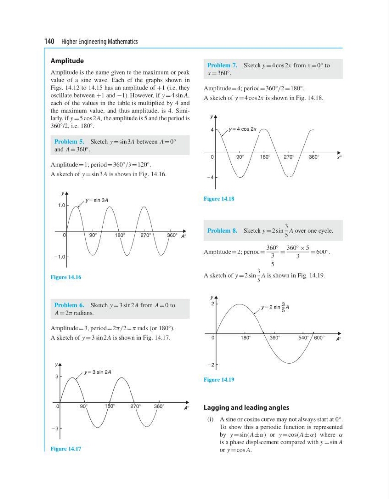
Amplitude= 1; period= 360 ◦ /3 =120 ◦ .
A sketch of y = sin 3 A is shown in Fig. 14.16.
y
1.0
21.0
0
908
2708
A8
1808
3608
y 5 sin 3A
Figure 14.16
Problem 6. Sketch y = 3 sin2A from A = 0 to
A = 2π radians.
Amplitude= 3, period= 2π/2 = π rads (or 180 ◦ ).
A sketch of y = 3 sin2A is shown in Fig. 14.17.
y
3
23
0
A8
y 5 3 sin 2A
2708
3608
1808
908
Figure 14.17
Problem 7. Sketch y = 4 cos2x from x = 0 ◦ to
x = 360 ◦ .
Amplitude= 4; period= 360 ◦ /2 =180 ◦ .
A sketch of y = 4 cos2x is shown in Fig. 14.18.
y
908
1808
2708
3608
x 8
0
24
4
y 5 4 cos 2x
Figure 14.18
Problem 8. Sketch y = 2 sin
3
5
A over one cycle.
Amplitude= 2; period=
360 ◦
3
5
=
360 ◦ × 5
3
= 600 ◦ .
A sketch of y = 2 sin
3
5
A is shown in Fig. 14.19.
1808
3608
5408 6008
y
A8
0
22
2
y 5 2 sin A
3
5
Figure 14.19
Lagging and leading angles
(i) A sine or cosine curve may not always start at 0 ◦ .
To show this a periodic function is represented
by y = sin(A ± α) or y = cos(A ± α) where α
is a phase displacement compared with y = sin A
or y = cos A.
Amplitude
Amplitude is the name given to the maximum or peak
value of a sine wave. Each of the graphs shown in
Figs. 14.12 to 14.15 has an amplitude of +1 (i.e. they
oscillate between +1 and −1). However, if y = 4 sin A,
each of the values in the table is multiplied by 4 and
the maximum value, and thus amplitude, is 4. Similarly, if y = 5 cos 2A, the amplitude is 5 and the period is
360 ◦ /2, i.e. 180 ◦ .
Problem 5. Sketch y = sin 3 A between A = 0 ◦
and A = 360 ◦ .
Amplitude= 1; period= 360 ◦ /3 =120 ◦ .
A sketch of y = sin 3 A is shown in Fig. 14.16.
y
1.0
21.0
0
908
2708
A8
1808
3608
y 5 sin 3A
Figure 14.16
Problem 6. Sketch y = 3 sin2A from A = 0 to
A = 2π radians.
Amplitude= 3, period= 2π/2 = π rads (or 180 ◦ ).
A sketch of y = 3 sin2A is shown in Fig. 14.17.
y
3
23
0
A8
y 5 3 sin 2A
2708
3608
1808
908
Figure 14.17
Problem 7. Sketch y = 4 cos2x from x = 0 ◦ to
x = 360 ◦ .
Amplitude= 4; period= 360 ◦ /2 =180 ◦ .
A sketch of y = 4 cos2x is shown in Fig. 14.18.
y
908
1808
2708
3608
x 8
0
24
4
y 5 4 cos 2x
Figure 14.18
Problem 8. Sketch y = 2 sin
3
5
A over one cycle.
Amplitude= 2; period=
360 ◦
3
5
=
360 ◦ × 5
3
= 600 ◦ .
A sketch of y = 2 sin
3
5
A is shown in Fig. 14.19.
1808
3608
5408 6008
y
A8
0
22
2
y 5 2 sin A
3
5
Figure 14.19
Lagging and leading angles
(i) A sine or cosine curve may not always start at 0 ◦ .
To show this a periodic function is represented
by y = sin(A ± α) or y = cos(A ± α) where α
is a phase displacement compared with y = sin A
or y = cos A.