

Analog and Digital Filters
661
P.6.2 Given the following fi lter’s transfer functions:
a. H jw
jw
jw a
a
( )ϭ
ϩ
for Ͼ 0
b. H jw
jw
w
jw
b jw w
b
( )
( )
( )
(
)
ϭ
ϩ
ϩ
ϩ
2
0
2
2
0
2
0
for
notch filter
Ͼ
Evaluate by hand:
a. The fi lter type
b. The gain at H(w = 0) and H(w = ∞)
c. The cutoff frequency w c
d. The gain at |H(w = w c )| and phase at H(w = w c )
e. The fi lter’s BW
P.6.3 Obtain the magnitude and phase plots for the transfer functions of P.6.1 for the following cases: a = 2, 6, and 10, and discuss the effect of a.
P.6.4 Obtain the magnitude and phase plots of the transfer functions of P.6.2 for the following cases:
a. a = 2, b = 2
b. a = 2, b = 5, and w o = 15
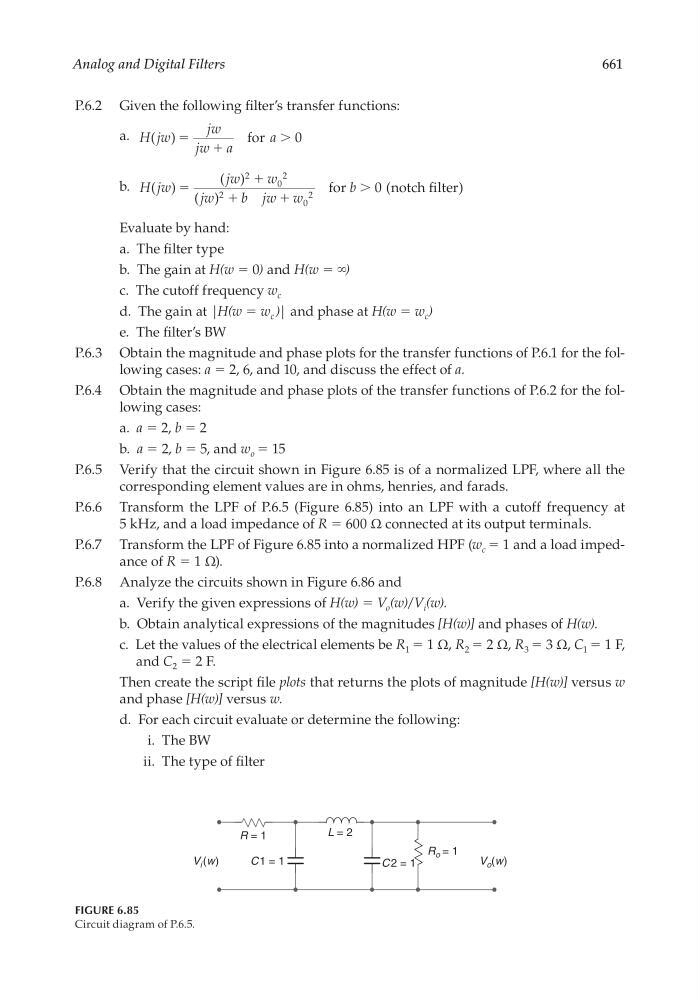
P.6.5 Verify that the circuit shown in Figure 6.85 is of a normalized LPF, where all the
corresponding element values are in ohms, henries, and farads.
P.6.6 Transform the LPF of P.6.5 (Figure 6.85) into an LPF with a cutoff frequency at
5 kHz, and a load impedance of R = 600 Ω connected at its output terminals.
P.6.7 Transform the LPF of Figure 6.85 into a normalized HPF (w c = 1 and a load impedance of R = 1 Ω).
P.6.8 Analyze the circuits shown in Figure 6.86 and
a. Verify the given expressions of H(w) = V o (w)/V i (w).
b. Obtain analytical expressions of the magnitudes [H(w)] and phases of H(w).
c. Let the values of the electrical elements be R 1 = 1 Ω, R 2 = 2 Ω, R 3 = 3 Ω, C 1 = 1 F,
and C 2 = 2 F.
Then create the script fi le plots that returns the plots of magnitude [H(w)] versus w
and phase [H(w)] versus w.
d. For each circuit evaluate or determine the following:
i. The BW
ii. The type of fi lter
FIGURE 6.85
Circuit diagram of P.6.5.
R = 1
R o = 1
C1 = 1
C 2 = 1
L = 2
V o (w)
V i (w)
CRC_47760_CH006.indd 661
CRC_47760_CH006.indd 661
7/23/2008 2:27:04 PM
7/23/2008 2:27:04 PM