660
Practical MATLAB
® Applications for Engineers
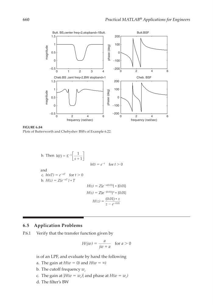
FIGURE 6.84
Plots of Butterworth and Chebyshev BSFs of Example 6.22.
0
1
2
3
4
0
−0.5
0
0.5
1
1.5
magnitude
−0.5
0
0.5
1
1.5
magnitude
Butt. BS,center freq=2,stopband=1Butt.
Butt.BSF
Cheb.BS ,cent freq=2,BW stopband=1
Cheb. BSF
0
2
4
6
0
2
4
6
−200
−100
100
200
phase (deg)
0
−200
−100
100
200
phase (deg)
frequency (rad/sec)
0
2
4
6
frequency (rad/sec)
b. Then h t
s
( ) ϭ
ϩ
Ϫ
£
1
1
1

 

 
h(t) = e
−t
for t > 0
and
c. h(nT) = e
−nT
for t > 0
b. H(z) = Z{e
−nT } * T
H(z) = Z{e
−n(0.01)
} * {0.01}
H(z) = Z{e
−(0.01)
}
n * {0.01}
H z
z
z e
( ) ϭ Ϫ
Ϫ
( . ) *
.
0 01
0 01
6.5 Application Problems
P.6.1 Verify that the transfer function given by
H jw
a
jw a
a
( ) ϭ
ϩ
for Ͼ 0
is of an LPF, and evaluate by hand the following
a. The gain at H(w = 0) and H(w = ∞)
b. The cutoff frequency w c
c. The gain at ͉H(w = w c )͉ and phase at H(w = w c )
d. The fi lter’s BW
CRC_47760_CH006.indd 660
CRC_47760_CH006.indd 660
7/23/2008 2:27:03 PM
7/23/2008 2:27:03 PM