Analog and Digital Filters
659
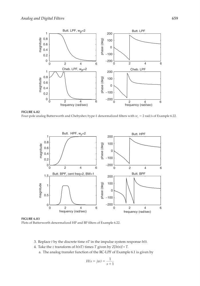
FIGURE 6.83
Plots of Butterworth denormalized HP and BP fi lters of Example 6.22.
Butt. HPF, w p =2
Butt. BPF, cent freq=2, BW=1
Butt. HPF
0
0.5
1
1.5
magnitude
Butt. BPF
0
2
4
6
0
0
2
4
6
0
2
4
6
0
2
4
6
−200
−100
0
100
200
phase (deg)
−200
−100
100
200
phase (deg)
0
0.2
0.4
0.6
0.8
1
magnitude
frequency (rad/sec)
frequency (rad/sec)
FIGURE 6.82
Four-pole analog Butterworth and Chebyshev/type-1 denormalized fi lters with w c = 2 rad/s of Example 6.22.
0
2
4
6
Butt. LPF, w p =2
0
2
4
6
−200
−100
0
0
100
200
phase (deg)
−200
−100
100
200
phase (deg)
Butt. LPF
Cheb. LPF
0
2
4
6
0
0.2
0.4
0.6
0.8
1
magnitude
0
0.2
0.4
0.6
0.8
1
magnitude
Cheb. LPF, w p =2
frequency (rad/sec)
0
2
4
6
frequency (rad/sec)
3. Replace t by the discrete time nT in the impulse system response h(t).
4. Take the z transform of h(nT) times T given by Z[h(n)] * T.
a. The analog transfer function of the RC-LPF of Example 6.1 is given by
H s jw
s
(
)
ϭ
ϭ ϩ
1
1
CRC_47760_CH006.indd 659
CRC_47760_CH006.indd 659
7/23/2008 2:27:02 PM
7/23/2008 2:27:02 PM