662
Practical MATLAB
® Applications for Engineers
iii. Regions of attenuation
iv. Regions of distortion
P.6.9 Design, at the circuit level, a Chebyshev type-1 and -2 BPF with w p = 2000 Hz connected to a load of R = 600 Ω. The schematic diagram is shown in Figure 6.87 and
verify that its transfer function is given by
H s
LC
s
s
CR LC
( ) ϭ
ϩ
ϩ
1
1
2
P.6.10 Obtain expressions of the 10th-order polynomials of the analog, Butterworth and
Chebyshev (types 1 and 2) LPFs with a cutoff frequency at 4 kHz.
P.6.11 Analyze the circuit diagram shown in Figure 6.88 and
a. Obtain the system transfer function.
b. Obtain plots of magnitude and phase of its transfer function for L = 1, and
C = 1/2.
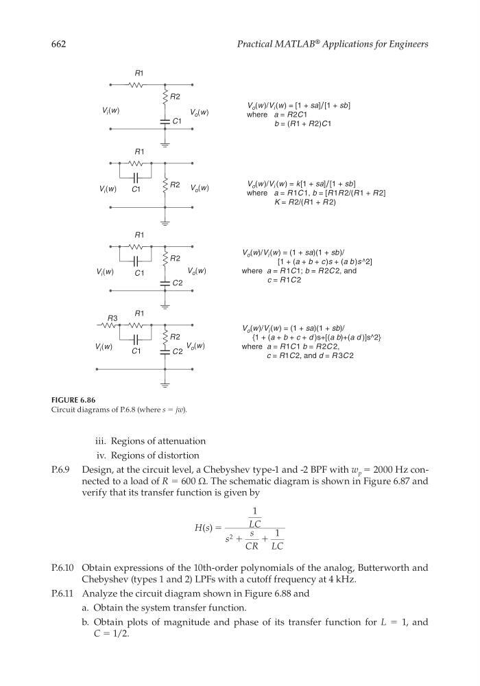
FIGURE 6.86
Circuit diagrams of P.6.8 (where s = jw).
R1
R2
C1
V i (w)
V i (w)
V o (w)
V o (w)
V i (w)
V o (w)
V i (w)
V o (w)
V o (w )/V i (w) = [1 + sa]/ [1 + sb]
where a = R 2C1
b = (R1 + R 2)C1
R1
R2
V o (w )/V i (w ) = k[1 + sa]/ [1 + sb]
where a = R 1C 1, b = [R 1R 2/(R 1 + R 2]
K = R 2/(R1 + R 2)
C1
R1
R 2
C2
R1
R2
V o (w)/V i (w) = (1 + sa)(1 + sb)/
[1 + (a + b + c )s + (a b )s ^2]
where a = R 1C1; b = R 2C 2, and
c = R 1C 2
C1
C1
C 2
R3
V o (w)/V i (w) = (1 + sa)(1 + sb)/
{1 + (a + b + c + d )s+[(a b)+(a d )]s^2}
where a = R1C 1 b = R 2C 2,
c = R1C 2, and d = R 3C 2
CRC_47760_CH006.indd 662
CRC_47760_CH006.indd 662
7/23/2008 2:27:04 PM
7/23/2008 2:27:04 PM