Analog and Digital Filters
629
Example 6.8
Create the script fi le direc_butt_disig that solves Example 6.7 by directly obtaining the
magnitude and phase plots of the discrete transfer function H(z) (LPF third order, with
T = 0.3 and a cutoff frequency of w c = 3 rad/s).
% Script file : direc _ butt _ disig
n =3;
T=.03;wc=3;w =-5:.1:5;
wz = w*T;
[Pz,Qz] = butter(n,wc*T/pi);
[magz,phasez]=freqz(Pz,Qz,wz/pi);
subplot(1,2,1)
plot(wz,magz);
title(‘Mag. of digital LPF’);axis([-5 5 0.4 1.1]);
xlabel(‘w in rad’)
ylabel(‘magnitude’)
subplot(1,2,2)
plot(wz,phasez*180/pi);
title(‘Phase of digital LPF vs w’)
xlabel(‘w in rad’)
ylabel(‘phase in degrees’)
Back in the command window, the script fi le direc_butt_disig is executed and the results
are shown as follows (Figure 6.58):
>> direc _ butt _ disig
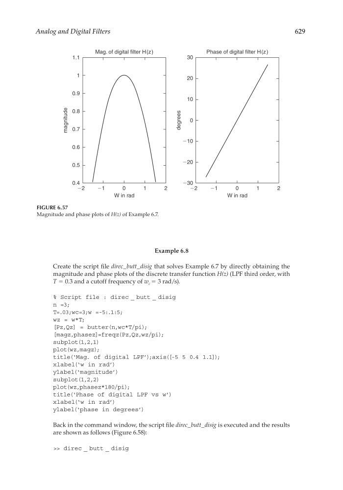
FIGURE 6.57
Magnitude and phase plots of H(z) of Example 6.7.
Mag. of digital filter H(z )
1
0.9
0.8
0.7
magnitude
0.6
0.5
1.1
0.4
Ϫ2
Ϫ1
0
1
2
W in rad
Phase of digital filter H(z )
30
20
10
Ϫ10
Ϫ20
Ϫ30
Ϫ2
Ϫ1
0
1
2
W in rad
0
degrees
CRC_47760_CH006.indd 629
CRC_47760_CH006.indd 629
7/23/2008 2:26:53 PM
7/23/2008 2:26:53 PM