628
Practical MATLAB
® Applications for Engineers
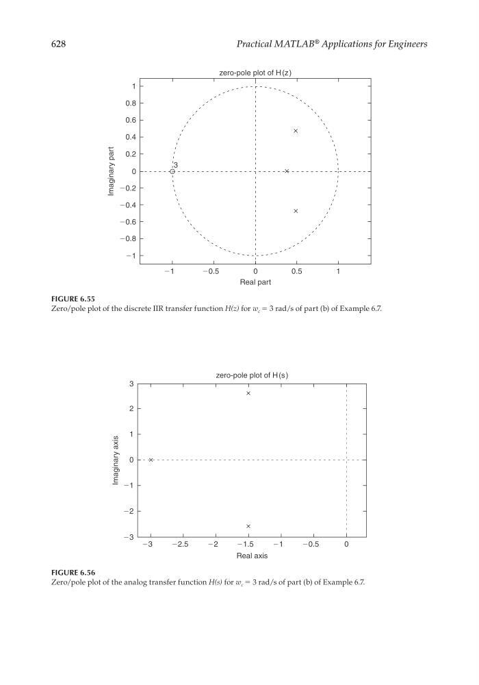
FIGURE 6.55
Zero/pole plot of the discrete IIR transfer function H(z) for w c = 3 rad/s of part (b) of Example 6.7.
1
zero-pole plot of H (z )
0.8
0.6
0.4
0.2
3
Ϫ0.2
Ϫ0.4
Ϫ0.6
Ϫ0.8
Ϫ1
Ϫ1
Ϫ0.5
0
0.5
1
Real part
0
Imaginary part
FIGURE 6.56
Zero/pole plot of the analog transfer function H(s) for w c = 3 rad/s of part (b) of Example 6.7.
3
zero-pole plot of H(s)
2
1
0
Ϫ1
Ϫ2
Ϫ3 Ϫ3
Ϫ2.5
Ϫ2
Ϫ1.5
Ϫ1
Ϫ0.5
0
Real axis
Imaginary axis
CRC_47760_CH006.indd 628
CRC_47760_CH006.indd 628
7/23/2008 2:26:53 PM
7/23/2008 2:26:53 PM