630
Practical MATLAB
® Applications for Engineers
Example 6.9
Create the script fi le cheby_HPF that returns the coeffi cients of the digital transfer function and the magnitude and phase plots of a third-order Chebyshev type-1 and -2 digital HPFs with the following specs:
1. w c = 0.5 rad/s
2. T = 0.3
3. R p = 2 dB
4. R s = 3 dB
MATLAB Solution
% Script file: cheby _ HPF
N =3;
% order
R p = 2; R s = 3;
% ripples
T = .3;
% sampling period
Wc = .5;
% cut off frequency
Wz = -2*pi:.01*pi:3*pi;
wzc = Wc*T/pi;
% normalized dig. frequency
[Pz1, Qz1] = cheby1(N, R p , wzc, ‘high’);
disp(‘********************************************’)
disp(‘*************R E S U L T S *****************’)
disp(‘********************************************’)
disp(‘For the transfer function H(z) of the Cheby/type1 HPF’)
disp(‘the numerators coefficients are:’)
disp(Pz1)
disp(‘The denominator coefficients are:’)
disp(Qz1)
[Pz2, Qz2] = cheby2(N, R s , wzc, ‘high’);
disp(‘ For the transfer function H(z) of the Cheby/type2 HPF’)
disp(‘The numerators coefficients are:’)
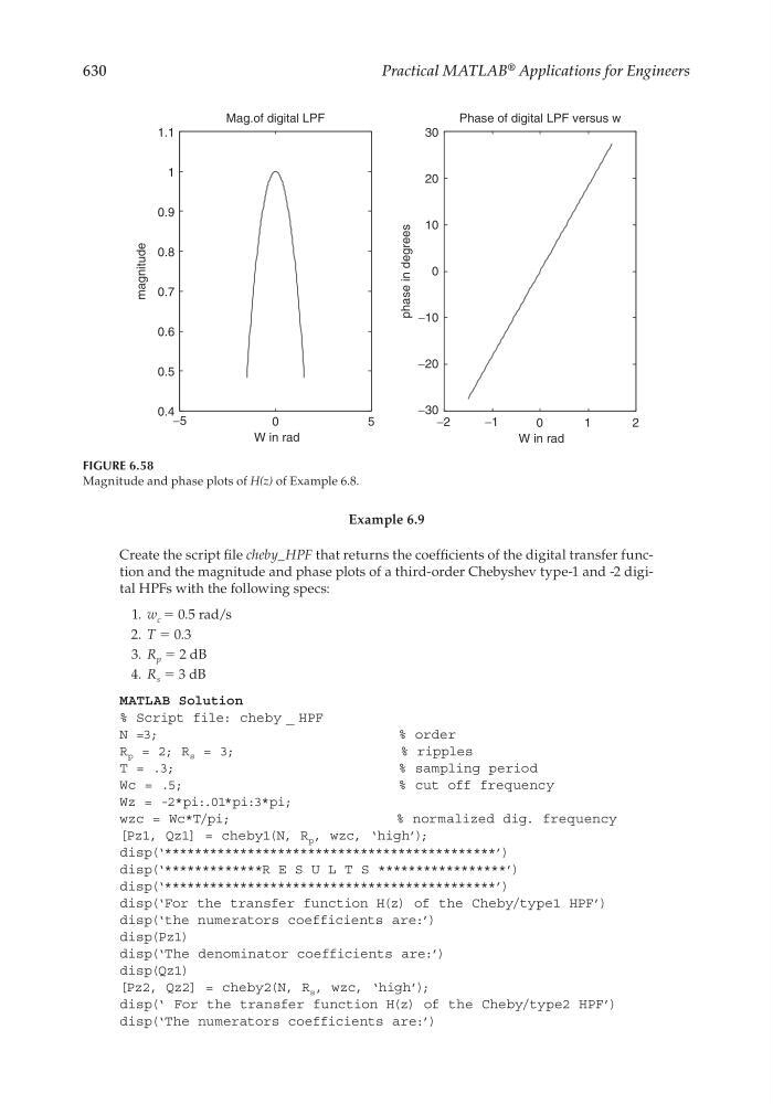
FIGURE 6.58
Magnitude and phase plots of H(z) of Example 6.8.
−5
0
5
0.4
0.5
0.6
0.7
0.8
0.9
1
1.1
Mag.of digital LPF
magnitude
−2
−1
0
1
2
−30
−20
−10
0
10
20
30
Phase of digital LPF versus w
W in rad
W in rad
phase in degrees
CRC_47760_CH006.indd 630
CRC_47760_CH006.indd 630
7/23/2008 2:26:53 PM
7/23/2008 2:26:53 PM