DTFT, DFT, ZT, and FFT
537
−15
−40
−30
−20
−10
0
10
20
30
40
−10
−5
0
Amplitude
5
10
15
20
Auto-correlation plots
R11
R22
R1
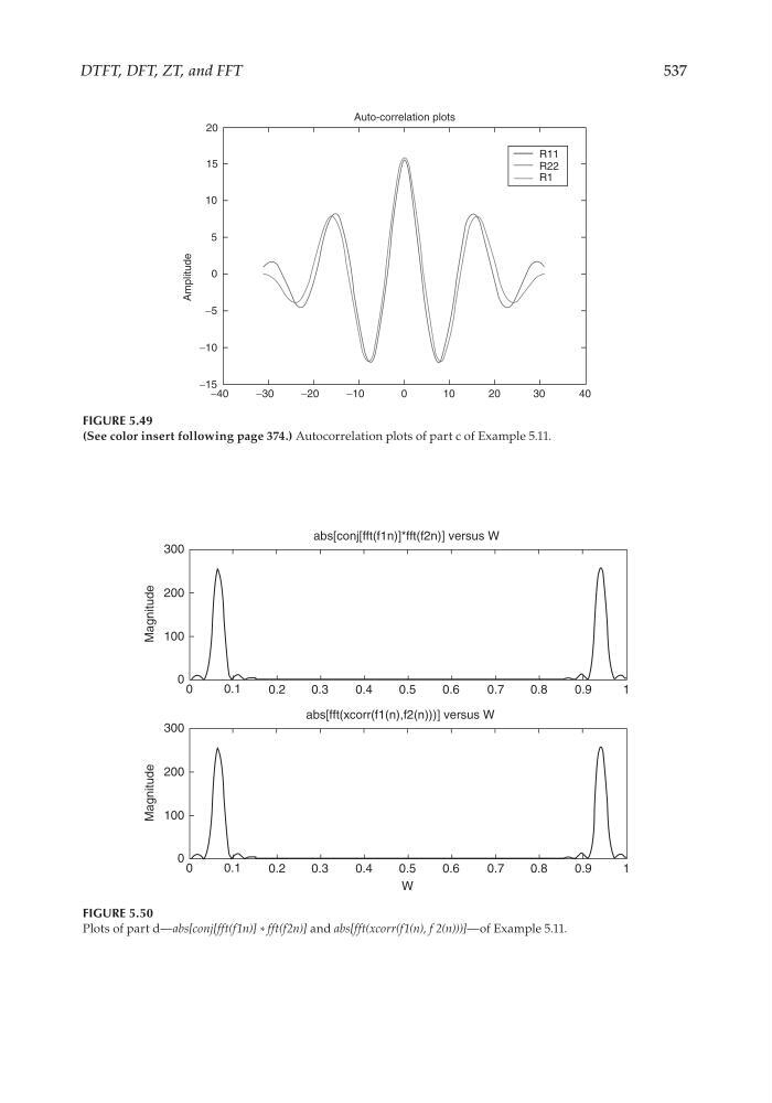
FIGURE 5.49
(See color insert following page 374.) Autocorrelation plots of part c of Example 5.11.
abs[conj[fft(f1n)]*fft(f2n)] versus W
abs[fft(xcorr(f1(n),f2(n)))] versus W
0
0
100
200
Magnitude
300
0.1
0.2
0.3
0.4
0.5
0.6
0.7
0.8
0.9
1
0
0
100
200
Magnitude
300
0.1
0.2
0.3
0.4
0.5
W
0.6
0.7
0.8
0.9
1
FIGURE 5.50
Plots of part d—abs[conj[fft(f1n)] * fft(f2n)] and abs[fft(xcorr(f1(n), f 2(n)))]—of Example 5.11.
CRC_47760_CH005.indd 537
CRC_47760_CH005.indd 537
7/23/2008 1:47:38 PM
7/23/2008 1:47:38 PM