538
Practical MATLAB
® Applications for Engineers
20
30
time index n
40
50
60
70
10
0
0
0.5
1
1.5
−10
20
30
40
50
60
70
10
0
−10
−4
−2
0
Amplitude
Amplitude
2
4
6
× 10 −15
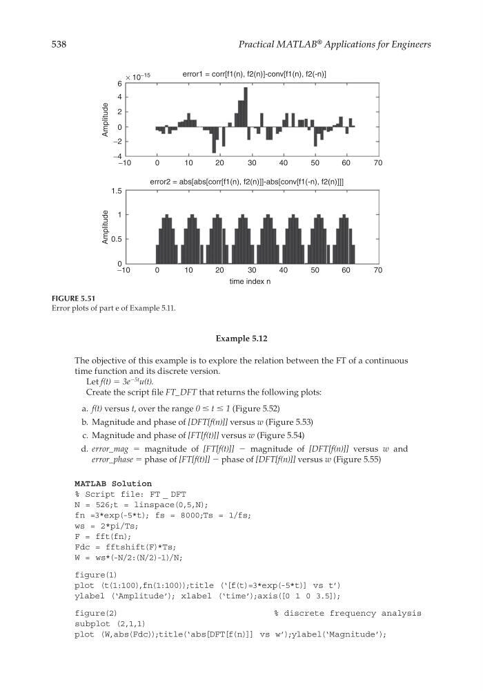
error2 = abs[abs[corr[f1(n), f2(n)]]-abs[conv[f1(-n), f2(n)]]]
error1 = corr[f1(n), f2(n)]-conv[f1(n), f2(-n)]
FIGURE 5.51
Error plots of part e of Example 5.11.
Example 5.12
The objective of this example is to explore the relation between the FT of a continuous
time function and its discrete version.
Let f(t) = 3e
−5t u(t).
Create the script fi le FT_DFT that returns the following plots:
a. f(t) versus t, over the range 0 ≤ t ≤ 1 (Figure 5.52)
b. Magnitude and phase of [DFT[f(n)]] versus w (Figure 5.53)
c. Magnitude and phase of [FT[f(t)]] versus w (Figure 5.54)
d. error_mag = magnitude of [FT[f(t)]] − magnitude of [DFT[f(n)]] versus w and
error_phase = phase of [FT[f(t)]] − phase of [DFT[f(n)]] versus w (Figure 5.55)
MATLAB Solution
% Script file: FT _ DFT
N = 526;t = linspace(0,5,N);
fn =3*exp(-5*t); fs = 8000;Ts = 1/fs;
ws = 2*pi/Ts;
F = fft(fn);
Fdc = fftshift(F)*Ts;
W = ws*(-N/2:(N/2)-1)/N;
figure(1)
plot (t(1:100),fn(1:100));title (‘[f(t)=3*exp(-5*t)] vs t’)
ylabel (‘Amplitude’); xlabel (‘time’);axis([0 1 0 3.5]);
figure(2)
% discrete frequency analysis
subplot (2,1,1)
plot (W,abs(Fdc));title(‘abs[DFT[f(n)]] vs w’);ylabel(‘Magnitude’);
CRC_47760_CH005.indd 538
CRC_47760_CH005.indd 538
7/23/2008 1:47:38 PM
7/23/2008 1:47:38 PM