536
Practical MATLAB
® Applications for Engineers
1
0.5
0
0
5
10
15
Stair plot of f1(n) versus n
20
25
30
Amplitude
−0.5
−1
1
0.5
0
0
5
10
15
time index n
Stair plot of f2(n) versus n
20
25
30
Amplitude
−0.5
−1
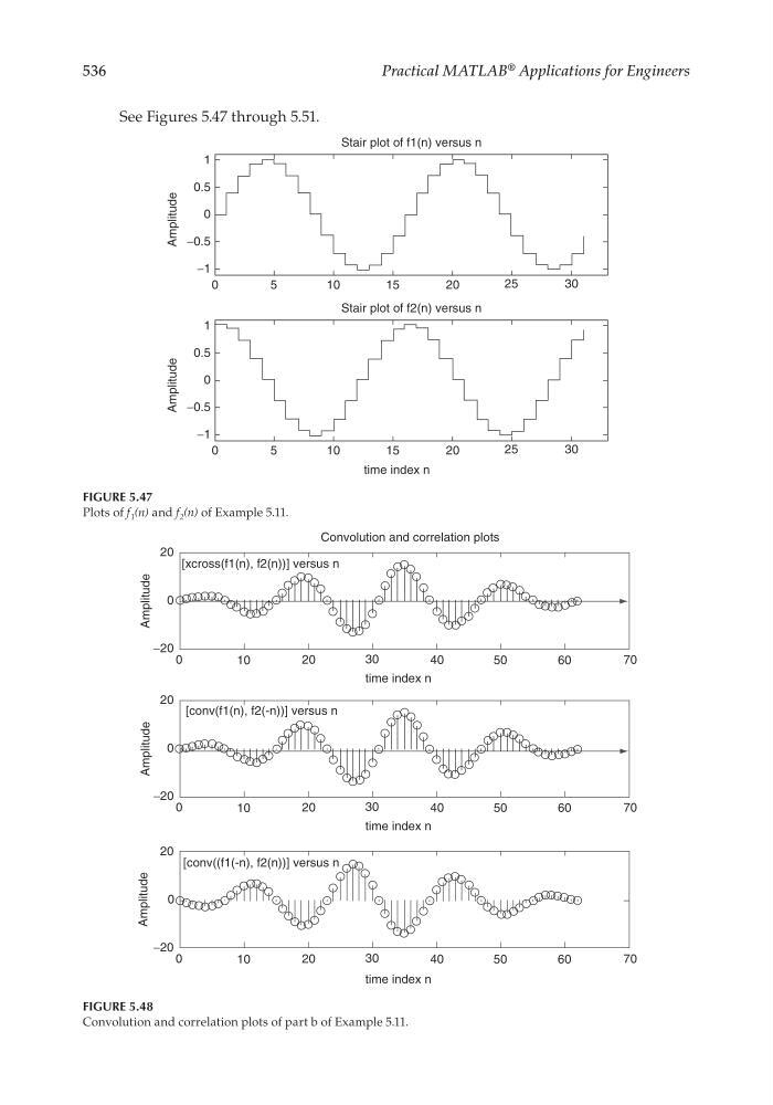
FIGURE 5.47
Plots of f 1 (n) and f 2 (n) of Example 5.11.
20
0
−20
0
10
20
30
40
50
60
70
20
0
−20
0
10
20
30
40
50
60
70
20
0
−20
0
10
20
30
40
50
60
70
time index n
time index n
time index n
Amplitude
Amplitude
Amplitude
Convolution and correlation plots
[xcross(f1(n), f2(n))] versus n
[conv(f1(n), f2(-n))] versus n
[conv((f1(-n), f2(n))] versus n
FIGURE 5.48
Convolution and correlation plots of part b of Example 5.11.
See Figures 5.47 through 5.51.
CRC_47760_CH005.indd 536
CRC_47760_CH005.indd 536
7/23/2008 1:47:37 PM
7/23/2008 1:47:37 PM