

414
Practical MATLAB
® Applications for Engineers
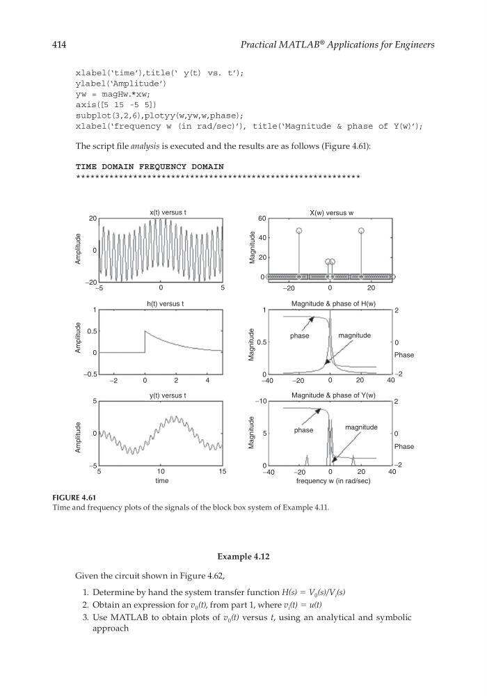
FIGURE 4.61
Time and frequency plots of the signals of the block box system of Example 4.11.
20
−20
−5
−2
1
5
0
0
−5
5
0
0
2
5
1 0
time
15
−40
−10
−20
−2
4
1
0.5
0
0.5
−0.5
h(t) versus t
y(t) versus t
x(t) versus t
X(w) versus w
0
0
2
0
5
20
40
−40
−20
−20
0
0
20
0
0
60
40
20
20
40
Phase
−2
0
2
Phase
phase
phase
frequency w (in rad/sec)
Magnitude & phase of Y(w)
Magnitude & phase of H(w)
magnitude
magnitude
Amplitude
Amplitude
Amplitude
Magnitude
Magnitude
Magnitude
xlabel(‘time’),title(‘ y(t) vs. t’);
ylabel(‘Amplitude’)
yw = magHw.*xw;
axis([5 15 -5 5])
subplot(3,2,6),plotyy(w,yw,w,phase);
xlabel(‘frequency w (in rad/sec)’), title(‘Magnitude & phase of Y(w)’);
The script fi le analysis is executed and the results are as follows (Figure 4.61):
TIME DOMAIN FREQUENCY DOMAIN
************************************************************
Example 4.12
Given the circuit shown in Figure 4.62,
1. Determine by hand the system transfer function H(s) = V 0 (s)/V i (s)
2. Obtain an expression for v 0 (t), from part 1, where v i (t) = u(t)
3. Use MATLAB to obtain plots of v 0 (t) versus t, using an analytical and symbolic
approach
CRC_47760_CH004.indd 414
CRC_47760_CH004.indd 414
7/28/2008 12:26:14 PM
7/28/2008 12:26:14 PM
Practical MATLAB
® Applications for Engineers
FIGURE 4.61
Time and frequency plots of the signals of the block box system of Example 4.11.
20
−20
−5
−2
1
5
0
0
−5
5
0
0
2
5
1 0
time
15
−40
−10
−20
−2
4
1
0.5
0
0.5
−0.5
h(t) versus t
y(t) versus t
x(t) versus t
X(w) versus w
0
0
2
0
5
20
40
−40
−20
−20
0
0
20
0
0
60
40
20
20
40
Phase
−2
0
2
Phase
phase
phase
frequency w (in rad/sec)
Magnitude & phase of Y(w)
Magnitude & phase of H(w)
magnitude
magnitude
Amplitude
Amplitude
Amplitude
Magnitude
Magnitude
Magnitude
xlabel(‘time’),title(‘ y(t) vs. t’);
ylabel(‘Amplitude’)
yw = magHw.*xw;
axis([5 15 -5 5])
subplot(3,2,6),plotyy(w,yw,w,phase);
xlabel(‘frequency w (in rad/sec)’), title(‘Magnitude & phase of Y(w)’);
The script fi le analysis is executed and the results are as follows (Figure 4.61):
TIME DOMAIN FREQUENCY DOMAIN
************************************************************
Example 4.12
Given the circuit shown in Figure 4.62,
1. Determine by hand the system transfer function H(s) = V 0 (s)/V i (s)
2. Obtain an expression for v 0 (t), from part 1, where v i (t) = u(t)
3. Use MATLAB to obtain plots of v 0 (t) versus t, using an analytical and symbolic
approach
CRC_47760_CH004.indd 414
CRC_47760_CH004.indd 414
7/28/2008 12:26:14 PM
7/28/2008 12:26:14 PM