

Fourier and Laplace
413
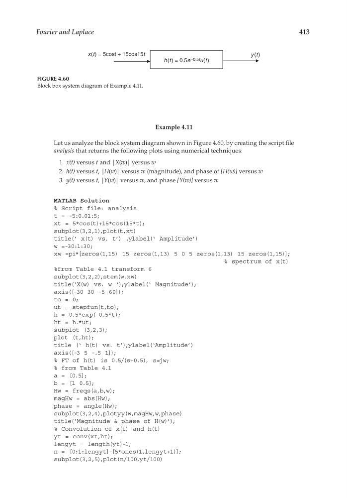
h (t ) = 0.5e −0.5t u(t )
x(t) = 5cost + 15cos15t
y (t )
FIGURE 4.60
Block box system diagram of Example 4.11.
Example 4.11
Let us analyze the block system diagram shown in Figure 4.60, by creating the script fi le
analysis that returns the following plots using numerical techniques:
1. x(t) versus t and |X(w)| versus w
2. h(t) versus t, |H(w)| versus w (magnitude), and phase of [H(w)] versus w
3. y(t) versus t, |Y(w)| versus w, and phase [Y(w)] versus w
MATLAB Solution
% Script file: analysis
t = -5:0.01:5;
xt = 5*cos(t)+15*cos(15*t);
subplot(3,2,1),plot(t,xt)
title(‘ x(t) vs. t’) ,ylabel(‘ Amplitude’)
w =-30:1:30;
xw =pi*[zeros(1,15) 15 zeros(1,13) 5 0 5 zeros(1,13) 15 zeros(1,15)];
% spectrum of x(t)
%from Table 4.1 transform 6
subplot(3,2,2),stem(w,xw)
title(‘X(w) vs. w ‘);ylabel(‘ Magnitude’);
axis([-30 30 -5 60]);
to = 0;
ut = stepfun(t,to);
h = 0.5*exp(-0.5*t);
ht = h.*ut;
subplot (3,2,3);
plot (t,ht);
title (‘ h(t) vs. t’);ylabel(‘Amplitude’)
axis([-3 5 -.5 1]);
% FT of h(t) is 0.5/(s+0.5), s=jw;
% from Table 4.1
a = [0.5];
b = [1 0.5];
Hw = freqs(a,b,w);
magHw = abs(Hw);
phase = angle(Hw);
subplot(3,2,4),plotyy(w,magHw,w,phase)
title(‘Magnitude & phase of H(w)’);
% Convolution of x(t) and h(t)
yt = conv(xt,ht);
lengyt = length(yt)-1;
n = [0:1:lengyt]-[5*ones(1,lengyt+1)];
subplot(3,2,5),plot(n/100,yt/100)
CRC_47760_CH004.indd 413
CRC_47760_CH004.indd 413
7/28/2008 12:26:14 PM
7/28/2008 12:26:14 PM
413
h (t ) = 0.5e −0.5t u(t )
x(t) = 5cost + 15cos15t
y (t )
FIGURE 4.60
Block box system diagram of Example 4.11.
Example 4.11
Let us analyze the block system diagram shown in Figure 4.60, by creating the script fi le
analysis that returns the following plots using numerical techniques:
1. x(t) versus t and |X(w)| versus w
2. h(t) versus t, |H(w)| versus w (magnitude), and phase of [H(w)] versus w
3. y(t) versus t, |Y(w)| versus w, and phase [Y(w)] versus w
MATLAB Solution
% Script file: analysis
t = -5:0.01:5;
xt = 5*cos(t)+15*cos(15*t);
subplot(3,2,1),plot(t,xt)
title(‘ x(t) vs. t’) ,ylabel(‘ Amplitude’)
w =-30:1:30;
xw =pi*[zeros(1,15) 15 zeros(1,13) 5 0 5 zeros(1,13) 15 zeros(1,15)];
% spectrum of x(t)
%from Table 4.1 transform 6
subplot(3,2,2),stem(w,xw)
title(‘X(w) vs. w ‘);ylabel(‘ Magnitude’);
axis([-30 30 -5 60]);
to = 0;
ut = stepfun(t,to);
h = 0.5*exp(-0.5*t);
ht = h.*ut;
subplot (3,2,3);
plot (t,ht);
title (‘ h(t) vs. t’);ylabel(‘Amplitude’)
axis([-3 5 -.5 1]);
% FT of h(t) is 0.5/(s+0.5), s=jw;
% from Table 4.1
a = [0.5];
b = [1 0.5];
Hw = freqs(a,b,w);
magHw = abs(Hw);
phase = angle(Hw);
subplot(3,2,4),plotyy(w,magHw,w,phase)
title(‘Magnitude & phase of H(w)’);
% Convolution of x(t) and h(t)
yt = conv(xt,ht);
lengyt = length(yt)-1;
n = [0:1:lengyt]-[5*ones(1,lengyt+1)];
subplot(3,2,5),plot(n/100,yt/100)
CRC_47760_CH004.indd 413
CRC_47760_CH004.indd 413
7/28/2008 12:26:14 PM
7/28/2008 12:26:14 PM