

Fourier and Laplace
415
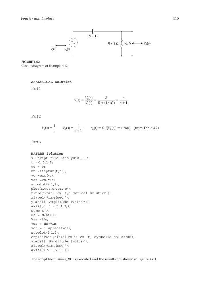
FIGURE 4.62
Circuit diagram of Example 4.12.
C = 1F
R = 1 Ω
V 0 (t )
V i (t )
V i (s)
V 0 (s)
ANALYTICAL Solution
Part 1
H s
V s
V s
R
R
sC
s
s
i
( )
( )
( )
( / )
ϭ
ϭ ϩ
ϭ ϩ
0
1
1
Part 2
V s
s
V s
s
v t
V s
e u t
i
t
( )
( )
( )
[ ( )]
( ) (
)
ϭ
ϭ
ϭ
ϭ
1
1
1
4
0
0
1
0
+
£
from Table .2
Ϫ
Ϫ
Part 3
MATLAB Solution
% Script file :analysis _ RC
t =-1:0.1:8;
t0 = 0;
ut =stepfun(t,t0);
vo =exp(-t);
vot =vo.*ut;
subplot(2,1,1);
plot(t,vot,t,vot,’o’);
title(‘vo(t) vs. t,numerical solution’);
xlabel(‘time(sec)’);
ylabel(‘ Amplitude (volts)’);
axis([-1 5 -.5 1.3]);
syms s x
Hs = s/(s+1);
Vis =1/s;
Vos = Hs*Vis;
vot = ilaplace(Vos);
subplot(2,1,2);
ezplot(vot);title(‘vo(t) vs. t, symbolic solution’);
ylabel(‘ Amplitude (volts)’);
xlabel(‘time(sec)’);
axis([0 5 -.5 1.3]);
The script fi le analysis_RC is executed and the results are shown in Figure 4.63.
CRC_47760_CH004.indd 415
CRC_47760_CH004.indd 415
7/28/2008 12:26:15 PM
7/28/2008 12:26:15 PM
415
FIGURE 4.62
Circuit diagram of Example 4.12.
C = 1F
R = 1 Ω
V 0 (t )
V i (t )
V i (s)
V 0 (s)
ANALYTICAL Solution
Part 1
H s
V s
V s
R
R
sC
s
s
i
( )
( )
( )
( / )
ϭ
ϭ ϩ
ϭ ϩ
0
1
1
Part 2
V s
s
V s
s
v t
V s
e u t
i
t
( )
( )
( )
[ ( )]
( ) (
)
ϭ
ϭ
ϭ
ϭ
1
1
1
4
0
0
1
0
+
£
from Table .2
Ϫ
Ϫ
Part 3
MATLAB Solution
% Script file :analysis _ RC
t =-1:0.1:8;
t0 = 0;
ut =stepfun(t,t0);
vo =exp(-t);
vot =vo.*ut;
subplot(2,1,1);
plot(t,vot,t,vot,’o’);
title(‘vo(t) vs. t,numerical solution’);
xlabel(‘time(sec)’);
ylabel(‘ Amplitude (volts)’);
axis([-1 5 -.5 1.3]);
syms s x
Hs = s/(s+1);
Vis =1/s;
Vos = Hs*Vis;
vot = ilaplace(Vos);
subplot(2,1,2);
ezplot(vot);title(‘vo(t) vs. t, symbolic solution’);
ylabel(‘ Amplitude (volts)’);
xlabel(‘time(sec)’);
axis([0 5 -.5 1.3]);
The script fi le analysis_RC is executed and the results are shown in Figure 4.63.
CRC_47760_CH004.indd 415
CRC_47760_CH004.indd 415
7/28/2008 12:26:15 PM
7/28/2008 12:26:15 PM