

258
Practical MATLAB
® Applications for Engineers
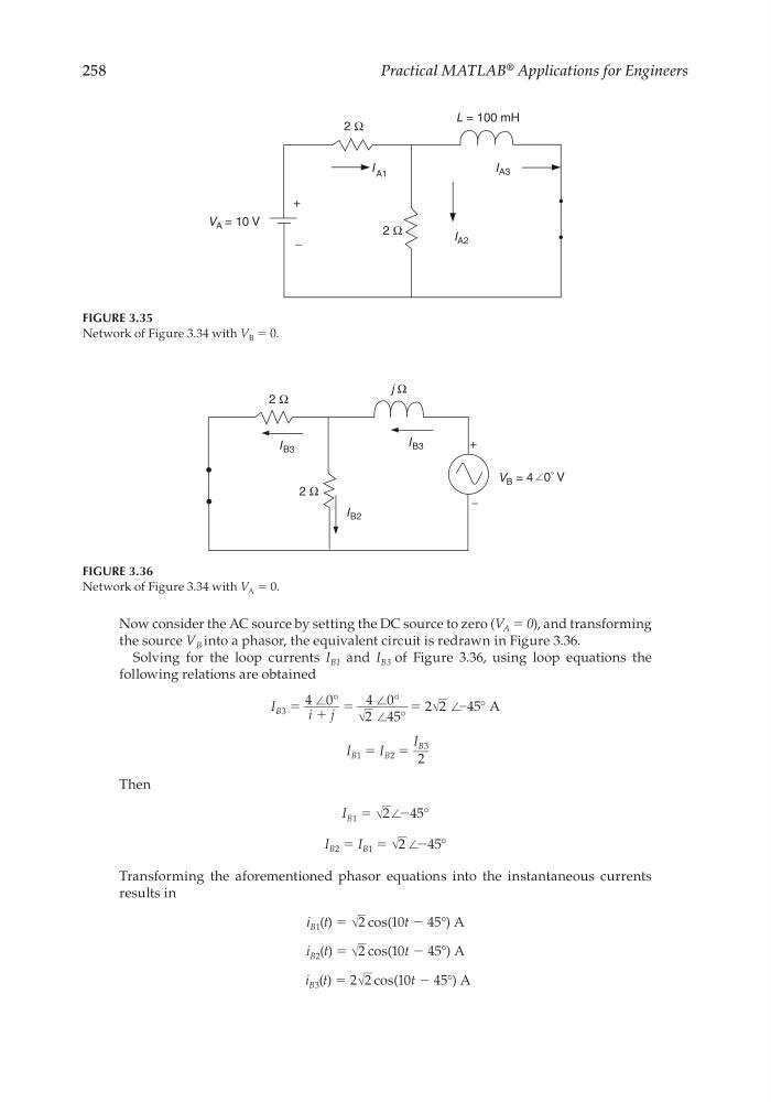
Now consider the AC source by setting the DC source to zero (V A = 0), and transforming
the source V B into a phasor, the equivalent circuit is redrawn in Figure 3.36.
Solving for the loop currents I B1 and I B3 of Figure 3.36, using loop equations the
following relations are obtained
I B3 = 4 ∠0°
______
i + j
= 4 ∠0°
________
√
__
2 ∠45°
= 2 √
__
2 ∠–45° A
I B1 = I B2 =
I B3
___
2
Then
I B1 = √
__
2 ∠−45°
I B2 = I B1 = √
__
2 ∠−45°
Transforming the aforementioned phasor equations into the instantaneous currents
results in
i B1 (t) = √
__
2 cos(10t − 45°) A
i B2 (t) = √
__
2 cos(10t − 45°) A
i B3 (t) = 2 √
__
2 cos(10t − 45°) A
V A = 10 V
I A3
I A2
L = 100 mH
2 Ω
2 Ω
I A1
+
−
FIGURE 3.35
Network of Figure 3.34 with V B = 0.
I B3
I B2
j Ω
2 Ω
2 Ω
I B3
+
V B = 4
−
0 ° V
FIGURE 3.36
Network of Figure 3.34 with V A = 0.
CRC_47760_CH003.indd 258
CRC_47760_CH003.indd 258
7/23/2008 1:27:40 PM
7/23/2008 1:27:40 PM
Practical MATLAB
® Applications for Engineers
Now consider the AC source by setting the DC source to zero (V A = 0), and transforming
the source V B into a phasor, the equivalent circuit is redrawn in Figure 3.36.
Solving for the loop currents I B1 and I B3 of Figure 3.36, using loop equations the
following relations are obtained
I B3 = 4 ∠0°
______
i + j
= 4 ∠0°
________
√
__
2 ∠45°
= 2 √
__
2 ∠–45° A
I B1 = I B2 =
I B3
___
2
Then
I B1 = √
__
2 ∠−45°
I B2 = I B1 = √
__
2 ∠−45°
Transforming the aforementioned phasor equations into the instantaneous currents
results in
i B1 (t) = √
__
2 cos(10t − 45°) A
i B2 (t) = √
__
2 cos(10t − 45°) A
i B3 (t) = 2 √
__
2 cos(10t − 45°) A
V A = 10 V
I A3
I A2
L = 100 mH
2 Ω
2 Ω
I A1
+
−
FIGURE 3.35
Network of Figure 3.34 with V B = 0.
I B3
I B2
j Ω
2 Ω
2 Ω
I B3
+
V B = 4
−
0 ° V
FIGURE 3.36
Network of Figure 3.34 with V A = 0.
CRC_47760_CH003.indd 258
CRC_47760_CH003.indd 258
7/23/2008 1:27:40 PM
7/23/2008 1:27:40 PM