

246
Practical MATLAB
® Applications for Engineers
and
2
2
1
1
2
2
ϭ
ϩ
ϩ
R
S
R
S
Q
Q
rad/s
if Q S > 10 then ω 1 = ω R ( 1 – 1
____
2Q S ) rad/s, and ω 2 = ω R ( 1 + 1
____
2Q S ) rad/s
where the BW is defi ned as BW = ω 2 − ω 1 or by BW = ω R /Q. Recall that the
BW represents the range of frequencies present in the output with a signifi cant
power content.
The frequency ω R is the geometric mean of the two frequencies given by ω 1
and ω 2 (or f 1 and f 2 ) as
R ϭ
1
2
⋅
or
f
f f
R ϭ 1 2
⋅
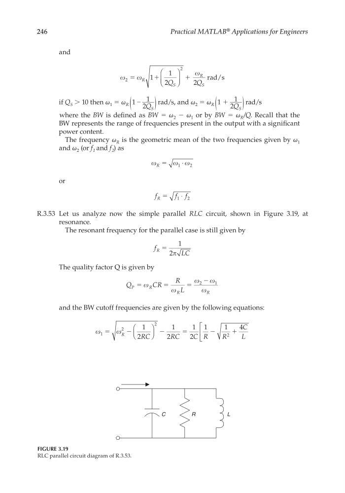
R.3.53 Let us analyze now the simple parallel RLC circuit, shown in Figure 3.19, at
resonance.
The resonant frequency for the parallel case is still given by
f
LC
R ϭ
1
2
The quality factor Q is given by
Q
C R
R
L
P
R
R
R
ϭ
ϭ
ϭ
Ϫ
2
1
and the BW cutoff frequencies are given by the following equations:
1
2
2
2
1
2
1
2
1
2
1
1
4
ϭ
Ϫ
Ϫ
ϭ
R
RC
RC
C R
R
C
L
Ϫ
ϩ
C
R
L
FIGURE 3.19
RLC parallel circuit diagram of R.3.53.
CRC_47760_CH003.indd 246
CRC_47760_CH003.indd 246
7/23/2008 1:27:36 PM
7/23/2008 1:27:36 PM
Practical MATLAB
® Applications for Engineers
and
2
2
1
1
2
2
ϭ
ϩ
ϩ
R
S
R
S
Q
Q
rad/s
if Q S > 10 then ω 1 = ω R ( 1 – 1
____
2Q S ) rad/s, and ω 2 = ω R ( 1 + 1
____
2Q S ) rad/s
where the BW is defi ned as BW = ω 2 − ω 1 or by BW = ω R /Q. Recall that the
BW represents the range of frequencies present in the output with a signifi cant
power content.
The frequency ω R is the geometric mean of the two frequencies given by ω 1
and ω 2 (or f 1 and f 2 ) as
R ϭ
1
2
⋅
or
f
f f
R ϭ 1 2
⋅
R.3.53 Let us analyze now the simple parallel RLC circuit, shown in Figure 3.19, at
resonance.
The resonant frequency for the parallel case is still given by
f
LC
R ϭ
1
2
The quality factor Q is given by
Q
C R
R
L
P
R
R
R
ϭ
ϭ
ϭ
Ϫ
2
1
and the BW cutoff frequencies are given by the following equations:
1
2
2
2
1
2
1
2
1
2
1
1
4
ϭ
Ϫ
Ϫ
ϭ
R
RC
RC
C R
R
C
L
Ϫ
ϩ
C
R
L
FIGURE 3.19
RLC parallel circuit diagram of R.3.53.
CRC_47760_CH003.indd 246
CRC_47760_CH003.indd 246
7/23/2008 1:27:36 PM
7/23/2008 1:27:36 PM