

168
X
M M
M
i
j
j
E
J
E
j i
m
2
2
¦
(9.2)
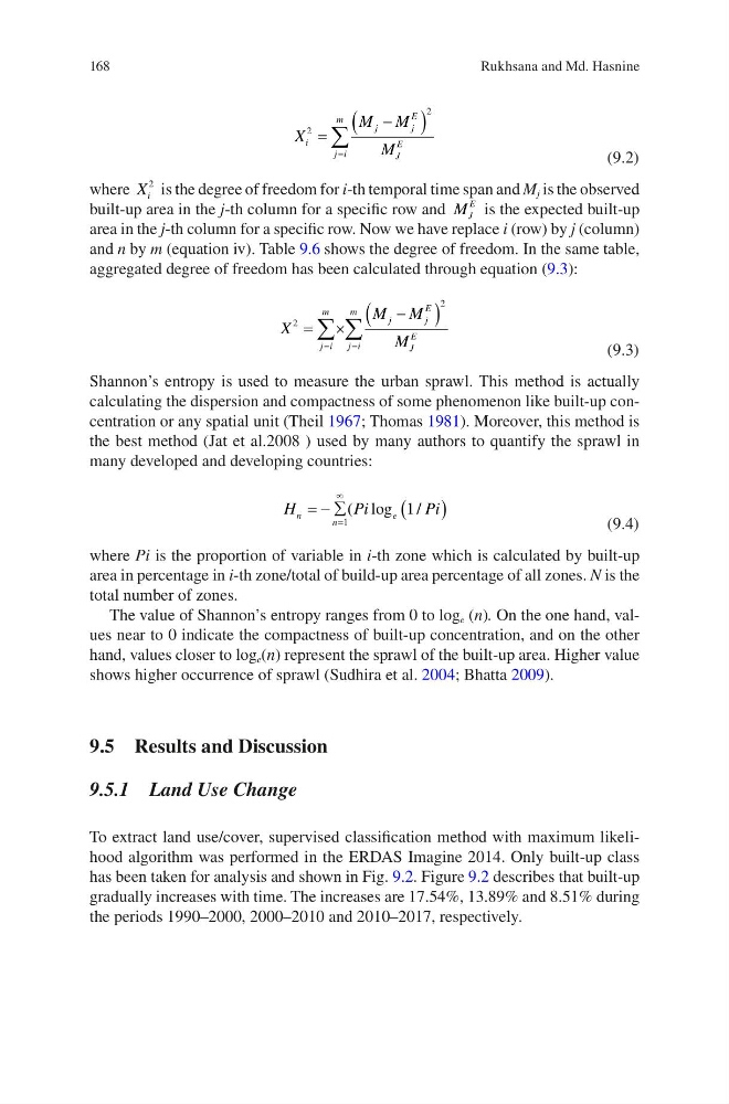
where X i
2 is the degree of freedom for i-th temporal time span and M j is the observed
built-up area in the j-th column for a specific row and M J
E is the expected built-up
area in the j-th column for a specific row. Now we have replace i (row) by j (column)
and n by m (equation iv). Table 9.6 shows the degree of freedom. In the same table,
aggregated degree of freedom has been calculated through equation (9.3):
X
M M
M
j i
m
j
j
E
J
E
j i
m
2
2
¦ ¦
u
(9.3)
Shannon’s entropy is used to measure the urban sprawl. This method is actually
calculating the dispersion and compactness of some phenomenon like built-up concentration or any spatial unit (Theil 1967; Thomas 1981). Moreover, this method is
the best method (Jat et al.2008 ) used by many authors to quantify the sprawl in
many developed and developing countries:
H
P i
P i
n
n
e
¦
f
1
1
( log /
(9.4)
where Pi is the proportion of variable in i-th zone which is calculated by built-up
area in percentage in i-th zone/total of build-up area percentage of all zones. N is the
total number of zones.
The value of Shannon’s entropy ranges from 0 to log e (n). On the one hand, values near to 0 indicate the compactness of built-up concentration, and on the other
hand, values closer to log e (n) represent the sprawl of the built-up area. Higher value
shows higher occurrence of sprawl (Sudhira et al. 2004; Bhatta 2009).
9.5 Results and Discussion
9.5.1 Land Use Change
To extract land use/cover, supervised classification method with maximum likelihood algorithm was performed in the ERDAS Imagine 2014. Only built-up class
has been taken for analysis and shown in Fig. 9.2. Figure 9.2 describes that built-up
gradually increases with time. The increases are 17.54%, 13.89% and 8.51% during
the periods 1990–2000, 2000–2010 and 2010–2017, respectively.
Rukhsana and Md. Hasnine
X
M M
M
i
j
j
E
J
E
j i
m
2
2
¦
(9.2)
where X i
2 is the degree of freedom for i-th temporal time span and M j is the observed
built-up area in the j-th column for a specific row and M J
E is the expected built-up
area in the j-th column for a specific row. Now we have replace i (row) by j (column)
and n by m (equation iv). Table 9.6 shows the degree of freedom. In the same table,
aggregated degree of freedom has been calculated through equation (9.3):
X
M M
M
j i
m
j
j
E
J
E
j i
m
2
2
¦ ¦
u
(9.3)
Shannon’s entropy is used to measure the urban sprawl. This method is actually
calculating the dispersion and compactness of some phenomenon like built-up concentration or any spatial unit (Theil 1967; Thomas 1981). Moreover, this method is
the best method (Jat et al.2008 ) used by many authors to quantify the sprawl in
many developed and developing countries:
H
P i
P i
n
n
e
¦
f
1
1
( log /
(9.4)
where Pi is the proportion of variable in i-th zone which is calculated by built-up
area in percentage in i-th zone/total of build-up area percentage of all zones. N is the
total number of zones.
The value of Shannon’s entropy ranges from 0 to log e (n). On the one hand, values near to 0 indicate the compactness of built-up concentration, and on the other
hand, values closer to log e (n) represent the sprawl of the built-up area. Higher value
shows higher occurrence of sprawl (Sudhira et al. 2004; Bhatta 2009).
9.5 Results and Discussion
9.5.1 Land Use Change
To extract land use/cover, supervised classification method with maximum likelihood algorithm was performed in the ERDAS Imagine 2014. Only built-up class
has been taken for analysis and shown in Fig. 9.2. Figure 9.2 describes that built-up
gradually increases with time. The increases are 17.54%, 13.89% and 8.51% during
the periods 1990–2000, 2000–2010 and 2010–2017, respectively.
Rukhsana and Md. Hasnine