

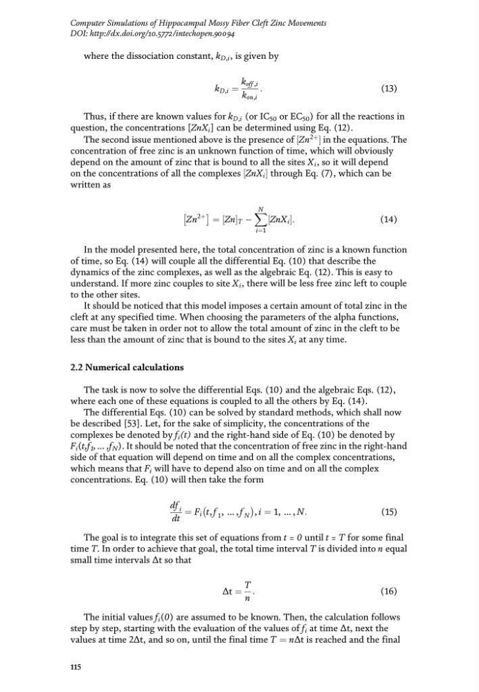
where the dissociation constant, k D,i , is given by
k D,i ¼
k off ,i
k on,i
:
(13)
Thus, if there are known values for k D,i (or IC 50 or EC 50 ) for all the reactions in
question, the concentrations [ZnX i ] can be determined using Eq. (12).
The second issue mentioned above is the presence of Zn
2þ
½� in the equations. The
concentration of free zinc is an unknown function of time, which will obviously
depend on the amount of zinc that is bound to all the sites X i , so it will depend
on the concentrations of all the complexes ZnX i
½� through Eq. (7), which can be
written as
Zn
2þ
��
¼ Zn
½� T �
X N
i¼1
ZnX i
½� :
(14)
In the model presented here, the total concentration of zinc is a known function
of time, so Eq. (14) will couple all the differential Eq. (10) that describe the
dynamics of the zinc complexes, as well as the algebraic Eq. (12). This is easy to
understand. If more zinc couples to site X i , there will be less free zinc left to couple
to the other sites.
It should be noticed that this model imposes a certain amount of total zinc in the
cleft at any specified time. When choosing the parameters of the alpha functions,
care must be taken in order not to allow the total amount of zinc in the cleft to be
less than the amount of zinc that is bound to the sites X i at any time.
2.2 Numerical calculations
The task is now to solve the differential Eqs. (10) and the algebraic Eqs. (12),
where each one of these equations is coupled to all the others by Eq. (14).
The differential Eqs. (10) can be solved by standard methods, which shall now
be described [53]. Let, for the sake of simplicity, the concentrations of the
complexes be denoted by f i (t) and the right-hand side of Eq. (10) be denoted by
F i (t,f 1 , … ,f N ). It should be noted that the concentration of free zinc in the right-hand
side of that equation will depend on time and on all the complex concentrations,
which means that F i will have to depend also on time and on all the complex
concentrations. Eq. (10) will then take the form
df i
dt
¼ F i t, f 1 , … , f N
�� , i ¼ 1, … , N:
(15)
The goal is to integrate this set of equations from t=0until t=Tfor some final
time T. In order to achieve that goal, the total time interval T is divided into n equal
small time intervals ∆t so that
∆t ¼
T
n
:
(16)
The initial values f i (0) are assumed to be known. Then, the calculation follows
step by step, starting with the evaluation of the values of f i at time ∆t, next the
values at time 2∆t, and so on, until the final time T ¼ n∆t is reached and the final
115
Computer Simulations of Hippocampal Mossy Fiber Cleft Zinc Movements
DOI: http://dx.doi.org/10.5772/intechopen.90094
k D,i ¼
k off ,i
k on,i
:
(13)
Thus, if there are known values for k D,i (or IC 50 or EC 50 ) for all the reactions in
question, the concentrations [ZnX i ] can be determined using Eq. (12).
The second issue mentioned above is the presence of Zn
2þ
½� in the equations. The
concentration of free zinc is an unknown function of time, which will obviously
depend on the amount of zinc that is bound to all the sites X i , so it will depend
on the concentrations of all the complexes ZnX i
½� through Eq. (7), which can be
written as
Zn
2þ
��
¼ Zn
½� T �
X N
i¼1
ZnX i
½� :
(14)
In the model presented here, the total concentration of zinc is a known function
of time, so Eq. (14) will couple all the differential Eq. (10) that describe the
dynamics of the zinc complexes, as well as the algebraic Eq. (12). This is easy to
understand. If more zinc couples to site X i , there will be less free zinc left to couple
to the other sites.
It should be noticed that this model imposes a certain amount of total zinc in the
cleft at any specified time. When choosing the parameters of the alpha functions,
care must be taken in order not to allow the total amount of zinc in the cleft to be
less than the amount of zinc that is bound to the sites X i at any time.
2.2 Numerical calculations
The task is now to solve the differential Eqs. (10) and the algebraic Eqs. (12),
where each one of these equations is coupled to all the others by Eq. (14).
The differential Eqs. (10) can be solved by standard methods, which shall now
be described [53]. Let, for the sake of simplicity, the concentrations of the
complexes be denoted by f i (t) and the right-hand side of Eq. (10) be denoted by
F i (t,f 1 , … ,f N ). It should be noted that the concentration of free zinc in the right-hand
side of that equation will depend on time and on all the complex concentrations,
which means that F i will have to depend also on time and on all the complex
concentrations. Eq. (10) will then take the form
df i
dt
¼ F i t, f 1 , … , f N
�� , i ¼ 1, … , N:
(15)
The goal is to integrate this set of equations from t=0until t=Tfor some final
time T. In order to achieve that goal, the total time interval T is divided into n equal
small time intervals ∆t so that
∆t ¼
T
n
:
(16)
The initial values f i (0) are assumed to be known. Then, the calculation follows
step by step, starting with the evaluation of the values of f i at time ∆t, next the
values at time 2∆t, and so on, until the final time T ¼ n∆t is reached and the final
115
Computer Simulations of Hippocampal Mossy Fiber Cleft Zinc Movements
DOI: http://dx.doi.org/10.5772/intechopen.90094