

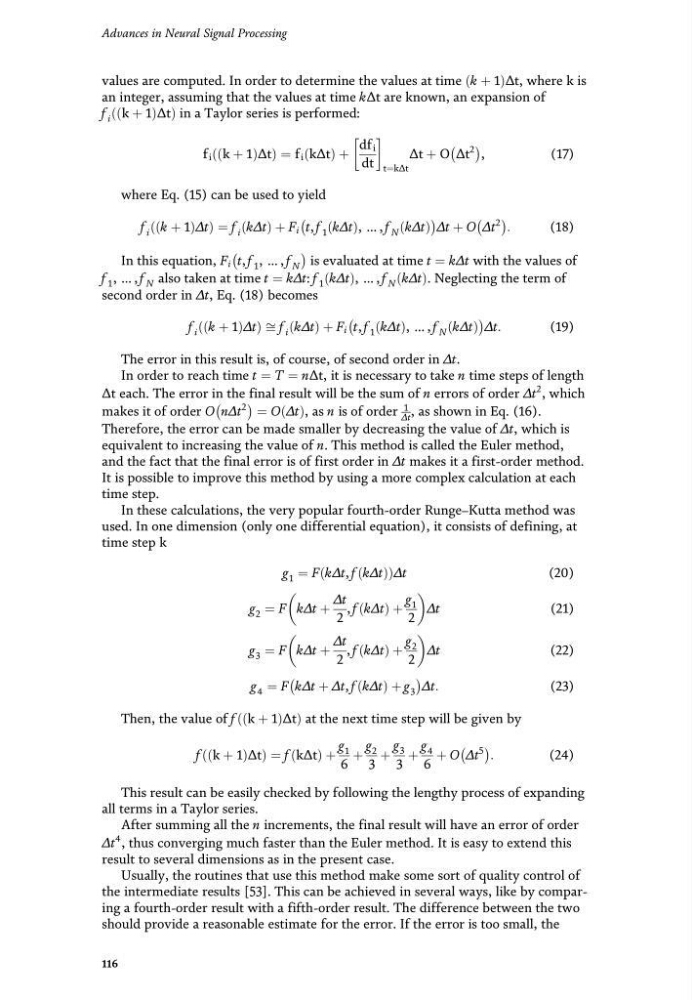
values are computed. In order to determine the values at time k þ 1
ðÞ ∆t, where k is
an integer, assuming that the values at time k∆t are known, an expansion of
f i k þ 1
ðÞ ∆t
ðÞ in a Taylor series is performed:
f i k þ 1
ðÞ ∆t
ð
Þ¼f i k∆t
ð
Þþ
df i
dt
t¼k∆t
∆t þ O ∆t
2
ÀÁ ,
(17)
where Eq. (15) can be used to yield
f i k þ 1
ðÞ ∆t
ð
Þ¼f i k∆t
ð ÞþF i t, f 1 k∆t
ðÞ , … , f N k∆t
ðÞ
ÀÁ
∆t þ O ∆t
2
ÀÁ
:
(18)
In this equation, F i t, f 1 , … , f N
ÀÁ is evaluated at time t ¼ k∆t with the values of
f 1 , … , f N also taken at time t ¼ k∆t: f 1 k∆t
ðÞ , … , f N k∆t
ðÞ . Neglecting the term of
second order in ∆t, Eq. (18) becomes
f i k þ 1
ðÞ ∆t
ð
Þffif i k∆t
ð ÞþF i t, f 1 k∆t
ðÞ , … , f N k∆t
ðÞ
ÀÁ
∆t:
(19)
The error in this result is, of course, of second order in ∆t.
In order to reach time t ¼ T ¼ n∆t, it is necessary to take n time steps of length
∆t each. The error in the final result will be the sum of n errors of order ∆t
2 , which
makes it of order On ∆t
2
ÀÁ
¼ O ∆t
ðÞ , as n is of order
1
∆t , as shown in Eq. (16).
Therefore, the error can be made smaller by decreasing the value of ∆t, which is
equivalent to increasing the value of n. This method is called the Euler method,
and the fact that the final error is of first order in ∆t makes it a first-order method.
It is possible to improve this method by using a more complex calculation at each
time step.
In these calculations, the very popular fourth-order Runge–Kutta method was
used. In one dimension (only one differential equation), it consists of defining, at
time step k
g 1 ¼ Fk ∆t, fk ∆t
ðÞ
ðÞ ∆t
(20)
g 2 ¼ Fk ∆t þ
∆t
2
, fk ∆t
ð Þþ
g 1
2
∆t
(21)
g 3 ¼ Fk ∆t þ
∆t
2
, fk ∆t
ð
Þþ
g 2
2
∆t
(22)
g 4 ¼ Fk ∆t þ ∆t, fk ∆t
ð
Þþg 3
ÀÁ
∆t:
(23)
Then, the value of f k þ 1
ðÞ ∆t
ðÞ at the next time step will be given by
f k þ 1
ðÞ ∆t
ð
Þ¼f k∆t
ð
Þþ
g 1
6
þ
g 2
3
þ
g 3
3
þ
g 4
6
þ O ∆t
5
ÀÁ
:
(24)
This result can be easily checked by following the lengthy process of expanding
all terms in a Taylor series.
After summing all the n increments, the final result will have an error of order
∆t
4 , thus converging much faster than the Euler method. It is easy to extend this
result to several dimensions as in the present case.
Usually, the routines that use this method make some sort of quality control of
the intermediate results [53]. This can be achieved in several ways, like by comparing a fourth-order result with a fifth-order result. The difference between the two
should provide a reasonable estimate for the error. If the error is too small, the
116
Advances in Neural Signal Processing
ðÞ ∆t, where k is
an integer, assuming that the values at time k∆t are known, an expansion of
f i k þ 1
ðÞ ∆t
ðÞ in a Taylor series is performed:
f i k þ 1
ðÞ ∆t
ð
Þ¼f i k∆t
ð
Þþ
df i
dt
t¼k∆t
∆t þ O ∆t
2
ÀÁ ,
(17)
where Eq. (15) can be used to yield
f i k þ 1
ðÞ ∆t
ð
Þ¼f i k∆t
ð ÞþF i t, f 1 k∆t
ðÞ , … , f N k∆t
ðÞ
ÀÁ
∆t þ O ∆t
2
ÀÁ
:
(18)
In this equation, F i t, f 1 , … , f N
ÀÁ is evaluated at time t ¼ k∆t with the values of
f 1 , … , f N also taken at time t ¼ k∆t: f 1 k∆t
ðÞ , … , f N k∆t
ðÞ . Neglecting the term of
second order in ∆t, Eq. (18) becomes
f i k þ 1
ðÞ ∆t
ð
Þffif i k∆t
ð ÞþF i t, f 1 k∆t
ðÞ , … , f N k∆t
ðÞ
ÀÁ
∆t:
(19)
The error in this result is, of course, of second order in ∆t.
In order to reach time t ¼ T ¼ n∆t, it is necessary to take n time steps of length
∆t each. The error in the final result will be the sum of n errors of order ∆t
2 , which
makes it of order On ∆t
2
ÀÁ
¼ O ∆t
ðÞ , as n is of order
1
∆t , as shown in Eq. (16).
Therefore, the error can be made smaller by decreasing the value of ∆t, which is
equivalent to increasing the value of n. This method is called the Euler method,
and the fact that the final error is of first order in ∆t makes it a first-order method.
It is possible to improve this method by using a more complex calculation at each
time step.
In these calculations, the very popular fourth-order Runge–Kutta method was
used. In one dimension (only one differential equation), it consists of defining, at
time step k
g 1 ¼ Fk ∆t, fk ∆t
ðÞ
ðÞ ∆t
(20)
g 2 ¼ Fk ∆t þ
∆t
2
, fk ∆t
ð Þþ
g 1
2
∆t
(21)
g 3 ¼ Fk ∆t þ
∆t
2
, fk ∆t
ð
Þþ
g 2
2
∆t
(22)
g 4 ¼ Fk ∆t þ ∆t, fk ∆t
ð
Þþg 3
ÀÁ
∆t:
(23)
Then, the value of f k þ 1
ðÞ ∆t
ðÞ at the next time step will be given by
f k þ 1
ðÞ ∆t
ð
Þ¼f k∆t
ð
Þþ
g 1
6
þ
g 2
3
þ
g 3
3
þ
g 4
6
þ O ∆t
5
ÀÁ
:
(24)
This result can be easily checked by following the lengthy process of expanding
all terms in a Taylor series.
After summing all the n increments, the final result will have an error of order
∆t
4 , thus converging much faster than the Euler method. It is easy to extend this
result to several dimensions as in the present case.
Usually, the routines that use this method make some sort of quality control of
the intermediate results [53]. This can be achieved in several ways, like by comparing a fourth-order result with a fifth-order result. The difference between the two
should provide a reasonable estimate for the error. If the error is too small, the
116
Advances in Neural Signal Processing