

SERVE-Boundary Conditions
311
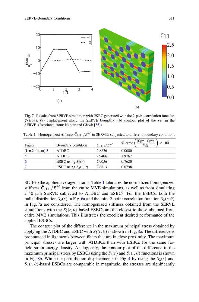
Fig. 7 Results from SERVE simulation with ESBC generated with the 2-point correlation function
S 2 (r, θ ): (a) displacement along the SERVE boundary, (b) contour plot of the 11 in the
SERVE. (Reprinted from: Kubair and Ghosh [35])
Table 1 Homogenized stiffness ¯
C 1111 /E M in SERVEs subjected to different boundary conditions
Figure
Boundary condition
¯
C 1111 /E M
% error
¯
C mve
1111 − ¯
C serve
1111
¯
C mve
1111
× 100
(L = 240 μm) 3
ATDBC
2.8836
0.0000
5
ATDBC
2.9406
1.9767
6
ESBC using S 2 (r)
2.9056
0.7620
7
ESBC using S 2 (r, θ)
2.8813
0.0798
SIGF to the applied averaged strains. Table 1 tabulates the normalized homogenized
stiffness ¯
C 1111 /E M from the entire MVE simulations, as well as from simulating
a 40 μm SERVE subjected to ATDBC and ESBCs. For the ESBCs, both the
radial distribution S 2 (r) in Fig. 6a and the joint 2-point correlation function S 2 (r, θ )
in Fig. 7a are considered. The homogenized stiffness obtained from the SERVE
simulations with the S 2 (r, θ )-based ESBCs are the closest to those obtained from
entire MVE simulations. This illustrates the excellent desired performance of the
applied ESBCs.
The contour plot of the difference in the maximum principal stress obtained by
applying the ATDBC and ESBC with S 2 (r, θ ) is shown in Fig. 8a. The difference is
pronounced in ligaments between fibers that are in close proximity. The maximum
principal stresses are larger with ATDBCs than with ESBCs for the same farfield strain energy density. Analogously, the contour plot of the difference in the
maximum principal stress by ESBCs using the S 2 (r) and S 2 (r, θ ) functions is shown
in Fig. 8b. While the perturbation displacements in Fig. 4 by using the S 2 (r) and
S 2 (r, θ )-based ESBCs are comparable in magnitude, the stresses are significantly
311
Fig. 7 Results from SERVE simulation with ESBC generated with the 2-point correlation function
S 2 (r, θ ): (a) displacement along the SERVE boundary, (b) contour plot of the 11 in the
SERVE. (Reprinted from: Kubair and Ghosh [35])
Table 1 Homogenized stiffness ¯
C 1111 /E M in SERVEs subjected to different boundary conditions
Figure
Boundary condition
¯
C 1111 /E M
% error
¯
C mve
1111 − ¯
C serve
1111
¯
C mve
1111
× 100
(L = 240 μm) 3
ATDBC
2.8836
0.0000
5
ATDBC
2.9406
1.9767
6
ESBC using S 2 (r)
2.9056
0.7620
7
ESBC using S 2 (r, θ)
2.8813
0.0798
SIGF to the applied averaged strains. Table 1 tabulates the normalized homogenized
stiffness ¯
C 1111 /E M from the entire MVE simulations, as well as from simulating
a 40 μm SERVE subjected to ATDBC and ESBCs. For the ESBCs, both the
radial distribution S 2 (r) in Fig. 6a and the joint 2-point correlation function S 2 (r, θ )
in Fig. 7a are considered. The homogenized stiffness obtained from the SERVE
simulations with the S 2 (r, θ )-based ESBCs are the closest to those obtained from
entire MVE simulations. This illustrates the excellent desired performance of the
applied ESBCs.
The contour plot of the difference in the maximum principal stress obtained by
applying the ATDBC and ESBC with S 2 (r, θ ) is shown in Fig. 8a. The difference is
pronounced in ligaments between fibers that are in close proximity. The maximum
principal stresses are larger with ATDBCs than with ESBCs for the same farfield strain energy density. Analogously, the contour plot of the difference in the
maximum principal stress by ESBCs using the S 2 (r) and S 2 (r, θ ) functions is shown
in Fig. 8b. While the perturbation displacements in Fig. 4 by using the S 2 (r) and
S 2 (r, θ )-based ESBCs are comparable in magnitude, the stresses are significantly