

310
S. Ghosh et al.
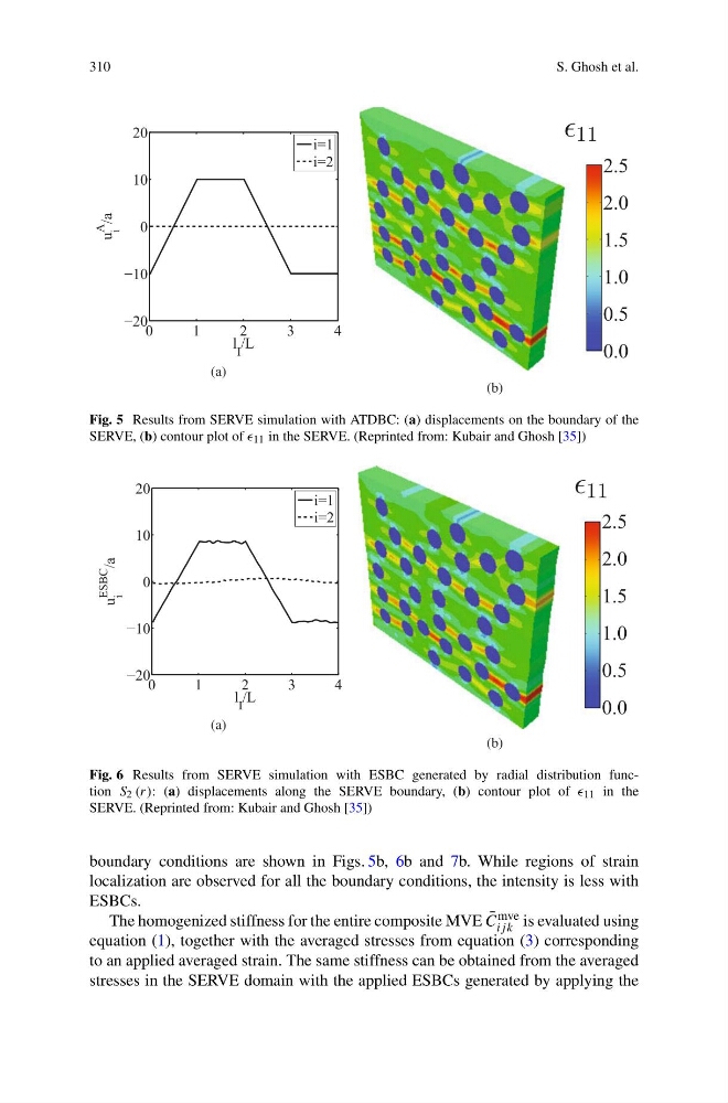
Fig. 5 Results from SERVE simulation with ATDBC: (a) displacements on the boundary of the
SERVE, (b) contour plot of 11 in the SERVE. (Reprinted from: Kubair and Ghosh [35])
Fig. 6 Results from SERVE simulation with ESBC generated by radial distribution function S 2 (r): (a) displacements along the SERVE boundary, (b) contour plot of 11 in the
SERVE. (Reprinted from: Kubair and Ghosh [35])
boundary conditions are shown in Figs. 5b, 6b and 7b. While regions of strain
localization are observed for all the boundary conditions, the intensity is less with
ESBCs.
The homogenized stiffness for the entire composite MVE ¯
C mve
ij k is evaluated using
equation (1), together with the averaged stresses from equation (3) corresponding
to an applied averaged strain. The same stiffness can be obtained from the averaged
stresses in the SERVE domain with the applied ESBCs generated by applying the
S. Ghosh et al.
Fig. 5 Results from SERVE simulation with ATDBC: (a) displacements on the boundary of the
SERVE, (b) contour plot of 11 in the SERVE. (Reprinted from: Kubair and Ghosh [35])
Fig. 6 Results from SERVE simulation with ESBC generated by radial distribution function S 2 (r): (a) displacements along the SERVE boundary, (b) contour plot of 11 in the
SERVE. (Reprinted from: Kubair and Ghosh [35])
boundary conditions are shown in Figs. 5b, 6b and 7b. While regions of strain
localization are observed for all the boundary conditions, the intensity is less with
ESBCs.
The homogenized stiffness for the entire composite MVE ¯
C mve
ij k is evaluated using
equation (1), together with the averaged stresses from equation (3) corresponding
to an applied averaged strain. The same stiffness can be obtained from the averaged
stresses in the SERVE domain with the applied ESBCs generated by applying the