

308
S. Ghosh et al.
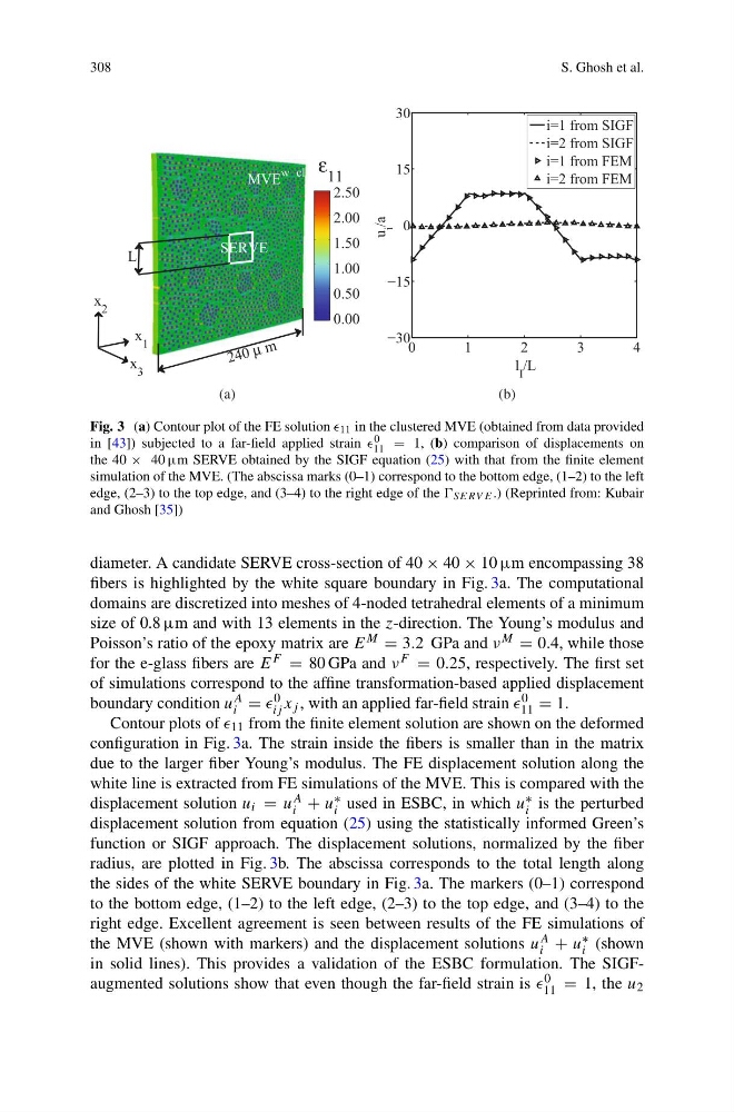
Fig. 3 (a) Contour plot of the FE solution 11 in the clustered MVE (obtained from data provided
in [43]) subjected to a far-field applied strain 0
11 = 1, (b) comparison of displacements on
the 40 × 40 μm SERVE obtained by the SIGF equation (25) with that from the finite element
simulation of the MVE. (The abscissa marks (0–1) correspond to the bottom edge, (1–2) to the left
edge, (2–3) to the top edge, and (3–4) to the right edge of the SERV E .) (Reprinted from: Kubair
and Ghosh [35])
diameter. A candidate SERVE cross-section of 40 × 40 × 10 μm encompassing 38
fibers is highlighted by the white square boundary in Fig. 3a. The computational
domains are discretized into meshes of 4-noded tetrahedral elements of a minimum
size of 0.8 μm and with 13 elements in the z-direction. The Young’s modulus and
Poisson’s ratio of the epoxy matrix are E M = 3.2 GPa and ν M = 0.4, while those
for the e-glass fibers are E F = 80 GPa and ν F = 0.25, respectively. The first set
of simulations correspond to the affine transformation-based applied displacement
boundary condition u A
i = 0
ij x j , with an applied far-field strain 0
11 = 1.
Contour plots of 11 from the finite element solution are shown on the deformed
configuration in Fig. 3a. The strain inside the fibers is smaller than in the matrix
due to the larger fiber Young’s modulus. The FE displacement solution along the
white line is extracted from FE simulations of the MVE. This is compared with the
displacement solution u i = u A
i + u ∗
i used in ESBC, in which u ∗
i is the perturbed
displacement solution from equation (25) using the statistically informed Green’s
function or SIGF approach. The displacement solutions, normalized by the fiber
radius, are plotted in Fig. 3b. The abscissa corresponds to the total length along
the sides of the white SERVE boundary in Fig. 3a. The markers (0–1) correspond
to the bottom edge, (1–2) to the left edge, (2–3) to the top edge, and (3–4) to the
right edge. Excellent agreement is seen between results of the FE simulations of
the MVE (shown with markers) and the displacement solutions u A
i + u ∗
i (shown
in solid lines). This provides a validation of the ESBC formulation. The SIGFaugmented solutions show that even though the far-field strain is 0
11 = 1, the u 2
S. Ghosh et al.
Fig. 3 (a) Contour plot of the FE solution 11 in the clustered MVE (obtained from data provided
in [43]) subjected to a far-field applied strain 0
11 = 1, (b) comparison of displacements on
the 40 × 40 μm SERVE obtained by the SIGF equation (25) with that from the finite element
simulation of the MVE. (The abscissa marks (0–1) correspond to the bottom edge, (1–2) to the left
edge, (2–3) to the top edge, and (3–4) to the right edge of the SERV E .) (Reprinted from: Kubair
and Ghosh [35])
diameter. A candidate SERVE cross-section of 40 × 40 × 10 μm encompassing 38
fibers is highlighted by the white square boundary in Fig. 3a. The computational
domains are discretized into meshes of 4-noded tetrahedral elements of a minimum
size of 0.8 μm and with 13 elements in the z-direction. The Young’s modulus and
Poisson’s ratio of the epoxy matrix are E M = 3.2 GPa and ν M = 0.4, while those
for the e-glass fibers are E F = 80 GPa and ν F = 0.25, respectively. The first set
of simulations correspond to the affine transformation-based applied displacement
boundary condition u A
i = 0
ij x j , with an applied far-field strain 0
11 = 1.
Contour plots of 11 from the finite element solution are shown on the deformed
configuration in Fig. 3a. The strain inside the fibers is smaller than in the matrix
due to the larger fiber Young’s modulus. The FE displacement solution along the
white line is extracted from FE simulations of the MVE. This is compared with the
displacement solution u i = u A
i + u ∗
i used in ESBC, in which u ∗
i is the perturbed
displacement solution from equation (25) using the statistically informed Green’s
function or SIGF approach. The displacement solutions, normalized by the fiber
radius, are plotted in Fig. 3b. The abscissa corresponds to the total length along
the sides of the white SERVE boundary in Fig. 3a. The markers (0–1) correspond
to the bottom edge, (1–2) to the left edge, (2–3) to the top edge, and (3–4) to the
right edge. Excellent agreement is seen between results of the FE simulations of
the MVE (shown with markers) and the displacement solutions u A
i + u ∗
i (shown
in solid lines). This provides a validation of the ESBC formulation. The SIGFaugmented solutions show that even though the far-field strain is 0
11 = 1, the u 2