

406
Compact Models for Integrated Circuit Design
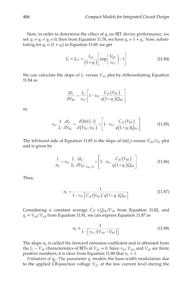
Now, in order to determine the effect of q e on BJT device performance, we
set: q c = q r = q f = 0; then from Equation 11.78, we have q b = 1 + q e . Now, substituting for q b = (1 + q e ) in Equation 11.69, we get
I
I
I
q
V
v
C
C T
SS
e
BE
kT
=
= +
(
)
−
1
1
exp
(11.84)
We can calculate the slope of I C versus V BE plot by differentiating Equation
11.84 as
dI
dV
I
v
v
C V
q
q Q
C
BE
C
kT
kT
jE
BE
e
B
=
−
( )
+
(
)
1
1
0
or,
v I
dI
dV
d
I
d V v
v
C V
q
q Q
kT
C
C
BE
C
BE
kT
kT
jE
BE
e
B
1
1
1
0
=
(
)
(
)
= −
( )
+
(
)
ln( )
(11.85)
The left-hand side of Equation 11.85 is the slope of ln(I C ) versus V BE /v kT plot
and is given by
1
1
1
1
0
0
n
v I
dI
dV
v
C V
q
q Q
E
kT
C
C
BE V
kT
jE
BE
e
B
BC
=
= −
( )
+
(
)
=
(11.86)
Thus,
n
v C V
q
q Q
E
kT
jE
BE
e
B
= −
( )
+
(
)
1
1
1
0
(11.87)
Considering a constant average C
Q V
jE
B
A R
= 0 /
from Equation 11.82, and
q e = V BE /V AR from Equation 11.81, we can express Equation 11.87 as
n
v
V
V
E
kT
AR
BE
≅ −
+
(
)
1
1
(11.88)
The slope n E is called the forward emission coefficient and is obtained from
the I C − V BE characteristics of BJTs at V BC = 0. Since v kT , V AR , and V BE are finite
positive numbers, it is clear from Equation 11.88 that n E > 1.
Evaluation of q c : The parameter q c models the base-width modulation due
to the applied CB-junction voltage V BC at the low current level during the
Compact Models for Integrated Circuit Design
Now, in order to determine the effect of q e on BJT device performance, we
set: q c = q r = q f = 0; then from Equation 11.78, we have q b = 1 + q e . Now, substituting for q b = (1 + q e ) in Equation 11.69, we get
I
I
I
q
V
v
C
C T
SS
e
BE
kT
=
= +
(
)
−
1
1
exp
(11.84)
We can calculate the slope of I C versus V BE plot by differentiating Equation
11.84 as
dI
dV
I
v
v
C V
q
q Q
C
BE
C
kT
kT
jE
BE
e
B
=
−
( )
+
(
)
1
1
0
or,
v I
dI
dV
d
I
d V v
v
C V
q
q Q
kT
C
C
BE
C
BE
kT
kT
jE
BE
e
B
1
1
1
0
=
(
)
(
)
= −
( )
+
(
)
ln( )
(11.85)
The left-hand side of Equation 11.85 is the slope of ln(I C ) versus V BE /v kT plot
and is given by
1
1
1
1
0
0
n
v I
dI
dV
v
C V
q
q Q
E
kT
C
C
BE V
kT
jE
BE
e
B
BC
=
= −
( )
+
(
)
=
(11.86)
Thus,
n
v C V
q
q Q
E
kT
jE
BE
e
B
= −
( )
+
(
)
1
1
1
0
(11.87)
Considering a constant average C
Q V
jE
B
A R
= 0 /
from Equation 11.82, and
q e = V BE /V AR from Equation 11.81, we can express Equation 11.87 as
n
v
V
V
E
kT
AR
BE
≅ −
+
(
)
1
1
(11.88)
The slope n E is called the forward emission coefficient and is obtained from
the I C − V BE characteristics of BJTs at V BC = 0. Since v kT , V AR , and V BE are finite
positive numbers, it is clear from Equation 11.88 that n E > 1.
Evaluation of q c : The parameter q c models the base-width modulation due
to the applied CB-junction voltage V BC at the low current level during the