

393
Bipolar Junction Transistor Compact Models
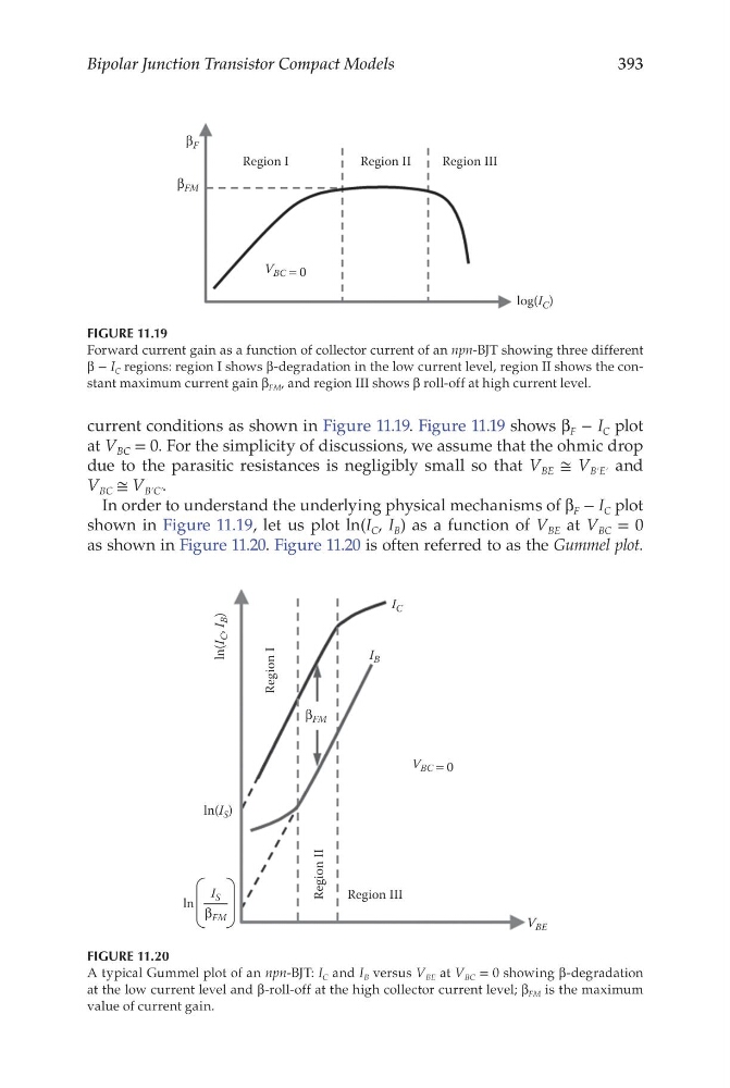
current conditions as shown in Figure 11.19. Figure 11.19 shows β F − I C plot
at V BC = 0. For the simplicity of discussions, we assume that the ohmic drop
due to the parasitic resistances is negligibly small so that V BE ≅ V B′E′ and
V BC ≅ V B′C′ .
In order to understand the underlying physical mechanisms of β F − I C plot
shown in Figure 11.19, let us plot ln(I C , I B ) as a function of V BE at V BC = 0
as shown in Figure 11.20. Figure 11.20 is often referred to as the Gummel plot.
Region I
Region II
Region III
V BC = 0
ln(I S )
ln(I
C , I
B )
β FM
I C
I B
V BE
β FM
I S
ln
FIGURE 11.20
A typical Gummel plot of an npn-BJT: I C and I B versus V BE at V BC = 0 showing β-degradation
at the low current level and β-roll-off at the high collector current level; β FM is the maximum
value of current gain.
Region I
R egion II
Region III
log(I C )
V BC = 0
β FM
β F
FIGURE 11.19
Forward current gain as a function of collector current of an npn-BJT showing three different
β − I C regions: region I shows β-degradation in the low current level, region II shows the constant maximum current gain β FM , and region III shows β roll-off at high current level.
Bipolar Junction Transistor Compact Models
current conditions as shown in Figure 11.19. Figure 11.19 shows β F − I C plot
at V BC = 0. For the simplicity of discussions, we assume that the ohmic drop
due to the parasitic resistances is negligibly small so that V BE ≅ V B′E′ and
V BC ≅ V B′C′ .
In order to understand the underlying physical mechanisms of β F − I C plot
shown in Figure 11.19, let us plot ln(I C , I B ) as a function of V BE at V BC = 0
as shown in Figure 11.20. Figure 11.20 is often referred to as the Gummel plot.
Region I
Region II
Region III
V BC = 0
ln(I S )
ln(I
C , I
B )
β FM
I C
I B
V BE
β FM
I S
ln
FIGURE 11.20
A typical Gummel plot of an npn-BJT: I C and I B versus V BE at V BC = 0 showing β-degradation
at the low current level and β-roll-off at the high collector current level; β FM is the maximum
value of current gain.
Region I
R egion II
Region III
log(I C )
V BC = 0
β FM
β F
FIGURE 11.19
Forward current gain as a function of collector current of an npn-BJT showing three different
β − I C regions: region I shows β-degradation in the low current level, region II shows the constant maximum current gain β FM , and region III shows β roll-off at high current level.