

381
Bipolar Junction Transistor Compact Models
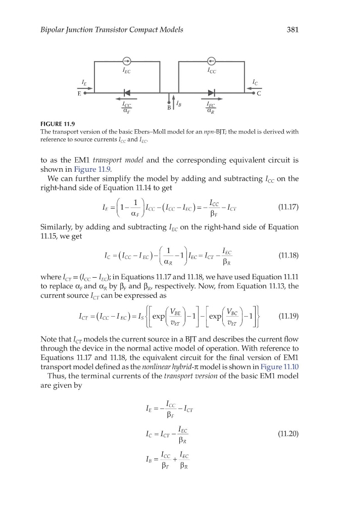
to as the EM1 transport model and the corresponding equivalent circuit is
shown in Figure 11.9.
We can further simplify the model by adding and subtracting I CC on the
right-hand side of Equation 11.14 to get
I
I
I
I
I
I
E
F
CC
CC
EC
CC
F
CT
= −
−
−
(
)=
−
1
1
α
β
−
(11.17)
Similarly, by adding and subtracting I EC on the right-hand side of Equation
11.15, we get
I
I
I
I
I
I
C
C C
E C
R
EC
CT
EC
R
=
−
(
)−
−
=
−
1 1
α
β
(11.18)
where I CT = (I CC − I EC ); in Equations 11.17 and 11.18, we have used Equation 11.11
to replace α F and α R by β F and β R , respectively. Now, from Equation 11.13, the
current source I CT can be expressed as
I
I
I
I
V
v
V
v
CT
CC
EC
S
BE
kT
BC
kT
=
−
(
)=
−
−
−
exp
e xp
1
1
(11.19)
Note that I CT models the current source in a BJT and describes the current flow
through the device in the normal active model of operation. With reference to
Equations 11.17 and 11.18, the equivalent circuit for the final version of EM1
transport model defined as the nonlinear hybrid-π model is shown in Figure 11.10
Thus, the terminal currents of the transport version of the basic EM1 model
are given by
I
I
I
I
I
I
I
I
I
E
CC
F
CT
C
C T
EC
R
B
CC
F
EC
R
= −
−
=
−
=
+
β
β
β
β
(11.20)
E
I E
I EC
I EC
B
I B
C
I C
I CC
I CC
α R
α F
FIGURE 11.9
The transport version of the basic Ebers–Moll model for an npn-BJT; the model is derived with
reference to source currents I CC and I EC .
Bipolar Junction Transistor Compact Models
to as the EM1 transport model and the corresponding equivalent circuit is
shown in Figure 11.9.
We can further simplify the model by adding and subtracting I CC on the
right-hand side of Equation 11.14 to get
I
I
I
I
I
I
E
F
CC
CC
EC
CC
F
CT
= −
−
−
(
)=
−
1
1
α
β
−
(11.17)
Similarly, by adding and subtracting I EC on the right-hand side of Equation
11.15, we get
I
I
I
I
I
I
C
C C
E C
R
EC
CT
EC
R
=
−
(
)−
−
=
−
1 1
α
β
(11.18)
where I CT = (I CC − I EC ); in Equations 11.17 and 11.18, we have used Equation 11.11
to replace α F and α R by β F and β R , respectively. Now, from Equation 11.13, the
current source I CT can be expressed as
I
I
I
I
V
v
V
v
CT
CC
EC
S
BE
kT
BC
kT
=
−
(
)=
−
−
−
exp
e xp
1
1
(11.19)
Note that I CT models the current source in a BJT and describes the current flow
through the device in the normal active model of operation. With reference to
Equations 11.17 and 11.18, the equivalent circuit for the final version of EM1
transport model defined as the nonlinear hybrid-π model is shown in Figure 11.10
Thus, the terminal currents of the transport version of the basic EM1 model
are given by
I
I
I
I
I
I
I
I
I
E
CC
F
CT
C
C T
EC
R
B
CC
F
EC
R
= −
−
=
−
=
+
β
β
β
β
(11.20)
E
I E
I EC
I EC
B
I B
C
I C
I CC
I CC
α R
α F
FIGURE 11.9
The transport version of the basic Ebers–Moll model for an npn-BJT; the model is derived with
reference to source currents I CC and I EC .