

335
Compact Models for Ultrathin Body FETs
Q K
E E
i
s i
s
s
=
−
(
)
ε 0 1
2
(9.56)
9.4.2 Drain Current Model
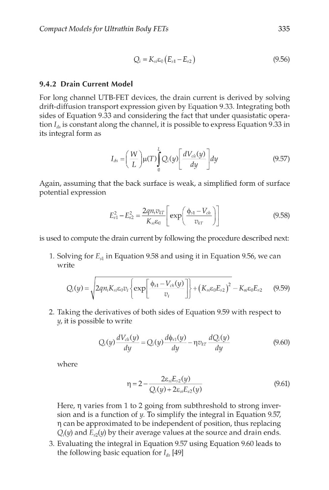
For long channel UTB-FET devices, the drain current is derived by solving
drift-diffusion transport expression given by Equation 9.33. Integrating both
sides of Equation 9.33 and considering the fact that under quasistatic operation I ds is constant along the channel, it is possible to express Equation 9.33 in
its integral form as
I
W
L
T Q y
dV y
dy
dy
ds
i
L
ch
=
∫
µ( )
( )
( )
0
(9.57)
Again, assuming that the back surface is weak, a simplified form of surface
potential expression
E E
qn v
K
V
v
s
s
i kT
si
s
c h
kT
1
2
2
2
0
1
2
−
=
−
ε
φ
exp
(9.58)
is used to compute the drain current by following the procedure described next:
1. Solving for E s1 in Equation 9.58 and using it in Equation 9.56, we can
write
Q y
qn K v
V y
v
K E
K
i
isi
t
s
c h
t
si
s
( )
exp
( )
=
−
+ (
) −
2
0
1
0 2
2
ε
φ
ε
s si
s
E
ε 0 2
(9.59)
2. Taking the derivatives of both sides of Equation 9.59 with respect to
y, it is possible to write
Q y
dV y
dy
Q y
d y
dy
v
dQ y
dy
i
ch
i
s
kT
i
( )
( )
( )
( )
( )
=
−
φ
η
1
(9.60)
where
η
ε
ε
= −
+
2
2
2
2
2
si s
i
s i s
E y
Q y
E y
( )
( )
( )
(9.61)
Here, η varies from 1 to 2 going from subthreshold to strong inversion and is a function of y. To simplify the integral in Equation 9.57,
η can be approximated to be independent of position, thus replacing
Q i (y) and E s2 (y) by their average values at the source and drain ends.
3. Evaluating the integral in Equation 9.57 using Equation 9.60 leads to
the following basic equation for I ds [49]
Compact Models for Ultrathin Body FETs
Q K
E E
i
s i
s
s
=
−
(
)
ε 0 1
2
(9.56)
9.4.2 Drain Current Model
For long channel UTB-FET devices, the drain current is derived by solving
drift-diffusion transport expression given by Equation 9.33. Integrating both
sides of Equation 9.33 and considering the fact that under quasistatic operation I ds is constant along the channel, it is possible to express Equation 9.33 in
its integral form as
I
W
L
T Q y
dV y
dy
dy
ds
i
L
ch
=
∫
µ( )
( )
( )
0
(9.57)
Again, assuming that the back surface is weak, a simplified form of surface
potential expression
E E
qn v
K
V
v
s
s
i kT
si
s
c h
kT
1
2
2
2
0
1
2
−
=
−
ε
φ
exp
(9.58)
is used to compute the drain current by following the procedure described next:
1. Solving for E s1 in Equation 9.58 and using it in Equation 9.56, we can
write
Q y
qn K v
V y
v
K E
K
i
isi
t
s
c h
t
si
s
( )
exp
( )
=
−
+ (
) −
2
0
1
0 2
2
ε
φ
ε
s si
s
E
ε 0 2
(9.59)
2. Taking the derivatives of both sides of Equation 9.59 with respect to
y, it is possible to write
Q y
dV y
dy
Q y
d y
dy
v
dQ y
dy
i
ch
i
s
kT
i
( )
( )
( )
( )
( )
=
−
φ
η
1
(9.60)
where
η
ε
ε
= −
+
2
2
2
2
2
si s
i
s i s
E y
Q y
E y
( )
( )
( )
(9.61)
Here, η varies from 1 to 2 going from subthreshold to strong inversion and is a function of y. To simplify the integral in Equation 9.57,
η can be approximated to be independent of position, thus replacing
Q i (y) and E s2 (y) by their average values at the source and drain ends.
3. Evaluating the integral in Equation 9.57 using Equation 9.60 leads to
the following basic equation for I ds [49]