

324
Compact Models for Integrated Circuit Design
β
ε
φ
≡
−
t
q
K v
n
N
y V y
v
fin
si
kT
i
b
ch
kT
2 2
0
2
0
exp
( )
( )
(9.29)
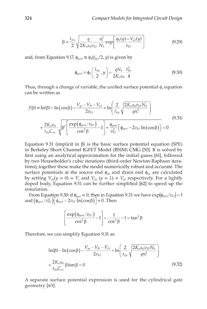
and, from Equation 9.17, f pert ≡ f 2 (t fin /2, y) is given by
φ
φ
ε
pert
fin
b
si
fin
t y
qN
K
t
≡
=
2
0
2
2
2
4
,
(9.30)
Thus, through a change of variable, the unified surface potential f s equation
can be written as
f
V V V
v
t
K v N
qn
gs
fb
ch
kT
fin
si
kT b
i
( ) ln( ) ln cos
l n
β
β
β
ε
≡
− (
)−
−
−
+
2
2 2
0
2
+
⋅
(
) −
+
2
1
0
2
2
K
t C
v
si
fin ox
pert
kT
pe
ε
β
φ
β
φ
exp
cos
r rt
kT
pert
kT
v
v
2
2
0
φ
β
−
(
)
=
ln cos
(9.31)
Equation 9.31 (implicit in β) is the basic surface potential equation (SPE)
in Berkeley Short Channel IGFET Model (BSIM) CMG [50]. It is solved by
first using an analytical approximation for the initial guess [61], followed
by two Householder’s cubic iterations (third-order Newton-Raphson iterations); together these make the model numerically robust and accurate. The
surface potentials at the source end f s0 and drain end f sL are calculated
by setting V ch (y = 0) = V s and V ch (y = L) = V d , respectively. For a lightly
doped body, Equation 9.31 can be further simplified [62] to speed up the
simulation.
From Equation 9.30: if f pert ≈ 0, then in Equation 9.31 we have exp φ pert kT
v
(
) = 1
and φ
φ
β
pert
kT
pert
kT
v
v
2
2
0
(
) −
(
)
≈
ln cos
. Then
exp
cos
c os
tan
φ
β
β
β
pert
kT
v
(
) −
=
− =
2
2
2
1
1
1
Therefore, we can simplify Equation 9.31 as
ln( ) ln cos
l n
β
β
ε
− (
)−
−
−
+
V V V
v
t
K v N
qn
gs
fb
ch
kT
fin
si
kT b
i
2
2 2
0
2
+
=
2
0
0
K
t C
si
fin ox
ε β
β
tan
(9.32)
A separate surface potential expression is used for the cylindrical gate
geometry [63].
Compact Models for Integrated Circuit Design
β
ε
φ
≡
−
t
q
K v
n
N
y V y
v
fin
si
kT
i
b
ch
kT
2 2
0
2
0
exp
( )
( )
(9.29)
and, from Equation 9.17, f pert ≡ f 2 (t fin /2, y) is given by
φ
φ
ε
pert
fin
b
si
fin
t y
qN
K
t
≡
=
2
0
2
2
2
4
,
(9.30)
Thus, through a change of variable, the unified surface potential f s equation
can be written as
f
V V V
v
t
K v N
qn
gs
fb
ch
kT
fin
si
kT b
i
( ) ln( ) ln cos
l n
β
β
β
ε
≡
− (
)−
−
−
+
2
2 2
0
2
+
⋅
(
) −
+
2
1
0
2
2
K
t C
v
si
fin ox
pert
kT
pe
ε
β
φ
β
φ
exp
cos
r rt
kT
pert
kT
v
v
2
2
0
φ
β
−
(
)
=
ln cos
(9.31)
Equation 9.31 (implicit in β) is the basic surface potential equation (SPE)
in Berkeley Short Channel IGFET Model (BSIM) CMG [50]. It is solved by
first using an analytical approximation for the initial guess [61], followed
by two Householder’s cubic iterations (third-order Newton-Raphson iterations); together these make the model numerically robust and accurate. The
surface potentials at the source end f s0 and drain end f sL are calculated
by setting V ch (y = 0) = V s and V ch (y = L) = V d , respectively. For a lightly
doped body, Equation 9.31 can be further simplified [62] to speed up the
simulation.
From Equation 9.30: if f pert ≈ 0, then in Equation 9.31 we have exp φ pert kT
v
(
) = 1
and φ
φ
β
pert
kT
pert
kT
v
v
2
2
0
(
) −
(
)
≈
ln cos
. Then
exp
cos
c os
tan
φ
β
β
β
pert
kT
v
(
) −
=
− =
2
2
2
1
1
1
Therefore, we can simplify Equation 9.31 as
ln( ) ln cos
l n
β
β
ε
− (
)−
−
−
+
V V V
v
t
K v N
qn
gs
fb
ch
kT
fin
si
kT b
i
2
2 2
0
2
+
=
2
0
0
K
t C
si
fin ox
ε β
β
tan
(9.32)
A separate surface potential expression is used for the cylindrical gate
geometry [63].