

323
Compact Models for Ultrathin Body FETs
E
qn
K
v
y
v
y
v
xs
i
si
kT
s
kT
kT
=
−
⋅
2
0
0
ε
φ
φ
exp
( ) exp
( ) e exp
( )
exp
( )
( )
− −
+
⋅
−
φ
φ
φ
φ
B
c h
kT
B
kT
s
V y
v
v
y
y
0
(9.25)
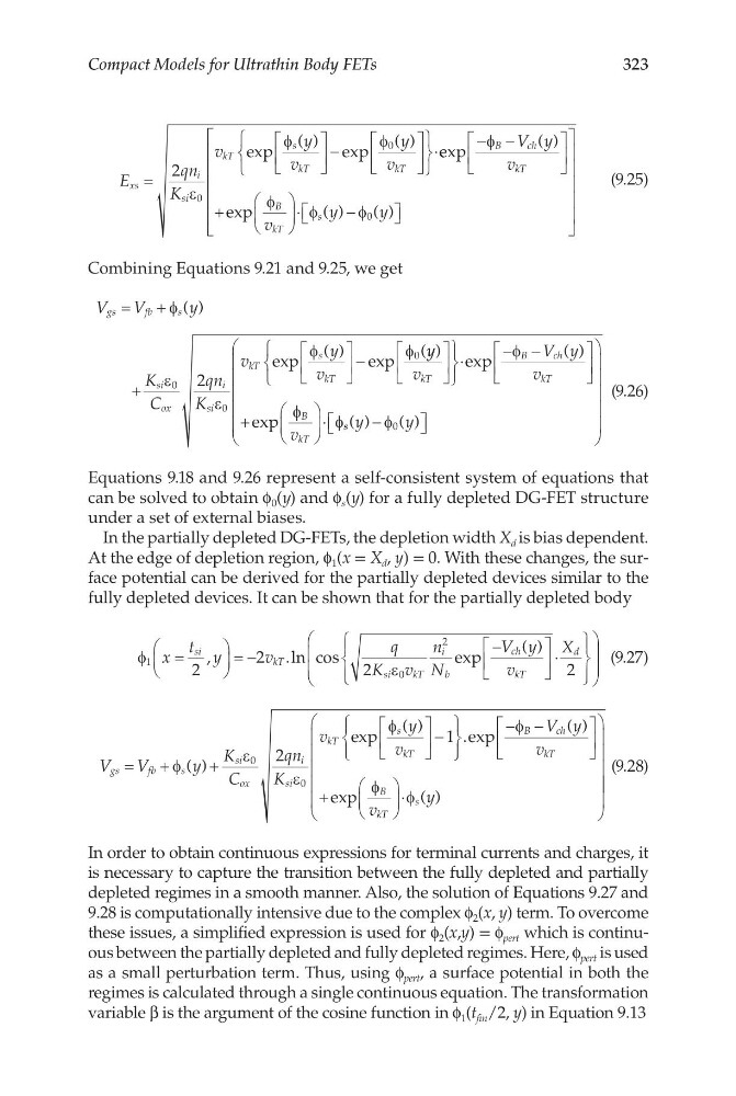
Combining Equations 9.21 and 9.25, we get
V
V
y
K
C
qn
K
v
y
v
gs
fb
s
si
ox
i
si
kT
s
kT
=
+
+
−
φ
ε
ε
φ
φ
( )
exp
( ) exp
(
0
0
0
2
y y
v
V y
v
v
kT
B
c h
kT
B
kT
) exp
( )
exp
⋅
− −
+
⋅
φ
φ
φ s s y
y
( )
( )
−
φ 0
(9.26)
Equations 9.18 and 9.26 represent a self-consistent system of equations that
can be solved to obtain f 0 (y) and f s (y) for a fully depleted DG-FET structure
under a set of external biases.
In the partially depleted DG-FETs, the depletion width X d is bias dependent.
At the edge of depletion region, f 1 (x = X d , y) = 0. With these changes, the surface potential can be derived for the partially depleted devices similar to the
fully depleted devices. It can be shown that for the partially depleted body
φ
ε
1
0
2
2
2
2
x
t y
v
q
K v
n
N
V y
v
si
kT
si
kT
i
b
ch
kT
=
= −
−
,
. ln cos
e xp
( )
⋅
X d
2
(9.27)
V
V
y
K
C
qn
K
v
y
v
gs
fb
s
si
ox
i
si
kT
s
kT
=
+
+
−
φ
ε
ε
φ
( )
exp
( )
0
0
2
1
− −
+
⋅
.exp
( )
exp
( )
φ
φ
φ
B
c h
kT
B
kT
s
V y
v
v
y
(9.28)
In order to obtain continuous expressions for terminal currents and charges, it
is necessary to capture the transition between the fully depleted and partially
depleted regimes in a smooth manner. Also, the solution of Equations 9.27 and
9.28 is computationally intensive due to the complex f 2 (x, y) term. To overcome
these issues, a simplified expression is used for f 2 (x,y) = f pert which is continuous between the partially depleted and fully depleted regimes. Here, f pert is used
as a small perturbation term. Thus, using f pert , a surface potential in both the
regimes is calculated through a single continuous equation. The transformation
variable β is the argument of the cosine function in f 1 (t fin /2, y) in Equation 9.13
Compact Models for Ultrathin Body FETs
E
qn
K
v
y
v
y
v
xs
i
si
kT
s
kT
kT
=
−
⋅
2
0
0
ε
φ
φ
exp
( ) exp
( ) e exp
( )
exp
( )
( )
− −
+
⋅
−
φ
φ
φ
φ
B
c h
kT
B
kT
s
V y
v
v
y
y
0
(9.25)
Combining Equations 9.21 and 9.25, we get
V
V
y
K
C
qn
K
v
y
v
gs
fb
s
si
ox
i
si
kT
s
kT
=
+
+
−
φ
ε
ε
φ
φ
( )
exp
( ) exp
(
0
0
0
2
y y
v
V y
v
v
kT
B
c h
kT
B
kT
) exp
( )
exp
⋅
− −
+
⋅
φ
φ
φ s s y
y
( )
( )
−
φ 0
(9.26)
Equations 9.18 and 9.26 represent a self-consistent system of equations that
can be solved to obtain f 0 (y) and f s (y) for a fully depleted DG-FET structure
under a set of external biases.
In the partially depleted DG-FETs, the depletion width X d is bias dependent.
At the edge of depletion region, f 1 (x = X d , y) = 0. With these changes, the surface potential can be derived for the partially depleted devices similar to the
fully depleted devices. It can be shown that for the partially depleted body
φ
ε
1
0
2
2
2
2
x
t y
v
q
K v
n
N
V y
v
si
kT
si
kT
i
b
ch
kT
=
= −
−
,
. ln cos
e xp
( )
⋅
X d
2
(9.27)
V
V
y
K
C
qn
K
v
y
v
gs
fb
s
si
ox
i
si
kT
s
kT
=
+
+
−
φ
ε
ε
φ
( )
exp
( )
0
0
2
1
− −
+
⋅
.exp
( )
exp
( )
φ
φ
φ
B
c h
kT
B
kT
s
V y
v
v
y
(9.28)
In order to obtain continuous expressions for terminal currents and charges, it
is necessary to capture the transition between the fully depleted and partially
depleted regimes in a smooth manner. Also, the solution of Equations 9.27 and
9.28 is computationally intensive due to the complex f 2 (x, y) term. To overcome
these issues, a simplified expression is used for f 2 (x,y) = f pert which is continuous between the partially depleted and fully depleted regimes. Here, f pert is used
as a small perturbation term. Thus, using f pert , a surface potential in both the
regimes is calculated through a single continuous equation. The transformation
variable β is the argument of the cosine function in f 1 (t fin /2, y) in Equation 9.13