

242
Compact Models for Integrated Circuit Design
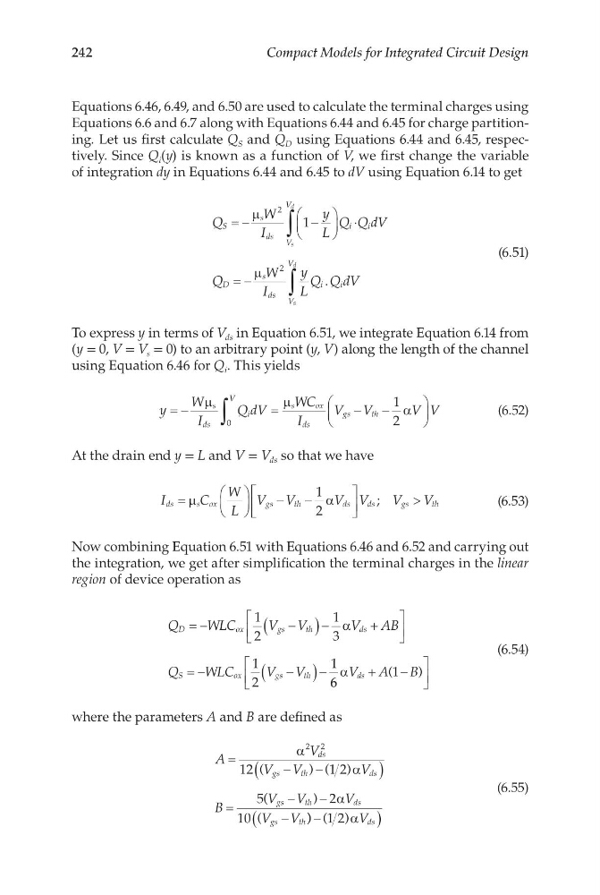
Equations 6.46, 6.49, and 6.50 are used to calculate the terminal charges using
Equations 6.6 and 6.7 along with Equations 6.44 and 6.45 for charge partitioning. Let us first calculate Q S and Q D using Equations 6.44 and 6.45, respectively. Since Q i (y) is known as a function of V, we first change the variable
of integration dy in Equations 6.44 and 6.45 to dV using Equation 6.14 to get
Q
W
I
y
L
Q Q dV
Q
W
I
y
L
Q Q dV
S
s
ds
i
V
V
i
D
s
ds
i
V
V
i
s
d
s
d
= −
−
⋅
= −
∫
∫
µ
µ
2
2
1
.
(6.51)
To express y in terms of V ds in Equation 6.51, we integrate Equation 6.14 from
(y = 0, V = V s = 0) to an arbitrary point (y, V) along the length of the channel
using Equation 6.46 for Q i . This yields
y
W
I
Q dV
WC
I
V V
V V
s
ds
i
V
s
o x
ds
gs
th
= −
=
−
−
∫
µ
µ
α
0
1
2
(6.52)
At the drain end y = L and V = V ds so that we have
I
C
W
L
V V
V V
V
V
ds
s ox
g s
t h
d s
d s
g s
t h
=
−
−
>
µ
α
1
2
;
(6.53)
Now combining Equation 6.51 with Equations 6.46 and 6.52 and carrying out
the integration, we get after simplification the terminal charges in the linear
region of device operation as
Q
WLC
V V
V AB
Q
WLC
V V
D
o x
g s
t h
d s
S
o x
g s
t h
= −
−
(
) −
+
= −
−
(
) −
1
2
1
3
1
2
1
α
6 6
1
αV A
B
ds +
−
(
)
(6.54)
where the parameters A and B are defined as
A
V
V V
V
B
V V
V
V V
ds
gs
th
ds
gs
th
ds
gs
th
=
−
−
(
)
=
−
−
−
α
α
α
2 2
12
1 2
5
2
10
(
) ( )
(
)
(
) ) ( )
−
(
)
1 2 αV ds
(6.55)
Compact Models for Integrated Circuit Design
Equations 6.46, 6.49, and 6.50 are used to calculate the terminal charges using
Equations 6.6 and 6.7 along with Equations 6.44 and 6.45 for charge partitioning. Let us first calculate Q S and Q D using Equations 6.44 and 6.45, respectively. Since Q i (y) is known as a function of V, we first change the variable
of integration dy in Equations 6.44 and 6.45 to dV using Equation 6.14 to get
Q
W
I
y
L
Q Q dV
Q
W
I
y
L
Q Q dV
S
s
ds
i
V
V
i
D
s
ds
i
V
V
i
s
d
s
d
= −
−
⋅
= −
∫
∫
µ
µ
2
2
1
.
(6.51)
To express y in terms of V ds in Equation 6.51, we integrate Equation 6.14 from
(y = 0, V = V s = 0) to an arbitrary point (y, V) along the length of the channel
using Equation 6.46 for Q i . This yields
y
W
I
Q dV
WC
I
V V
V V
s
ds
i
V
s
o x
ds
gs
th
= −
=
−
−
∫
µ
µ
α
0
1
2
(6.52)
At the drain end y = L and V = V ds so that we have
I
C
W
L
V V
V V
V
V
ds
s ox
g s
t h
d s
d s
g s
t h
=
−
−
>
µ
α
1
2
;
(6.53)
Now combining Equation 6.51 with Equations 6.46 and 6.52 and carrying out
the integration, we get after simplification the terminal charges in the linear
region of device operation as
Q
WLC
V V
V AB
Q
WLC
V V
D
o x
g s
t h
d s
S
o x
g s
t h
= −
−
(
) −
+
= −
−
(
) −
1
2
1
3
1
2
1
α
6 6
1
αV A
B
ds +
−
(
)
(6.54)
where the parameters A and B are defined as
A
V
V V
V
B
V V
V
V V
ds
gs
th
ds
gs
th
ds
gs
th
=
−
−
(
)
=
−
−
−
α
α
α
2 2
12
1 2
5
2
10
(
) ( )
(
)
(
) ) ( )
−
(
)
1 2 αV ds
(6.55)