

240
Compact Models for Integrated Circuit Design
∂ ′
∂ ′
′ = −
∂
′
∂
′
−
=−
∂
∫
∫
I y t
y
dy
W
Q y t
t
dy
I y t I t
W
Q
y
i
y
i
( , )
( , )
( , ) ( , )
0
0
0
or
( ( , )
′
∂
′
∫
y t
t
dy
y
0
(6.41)
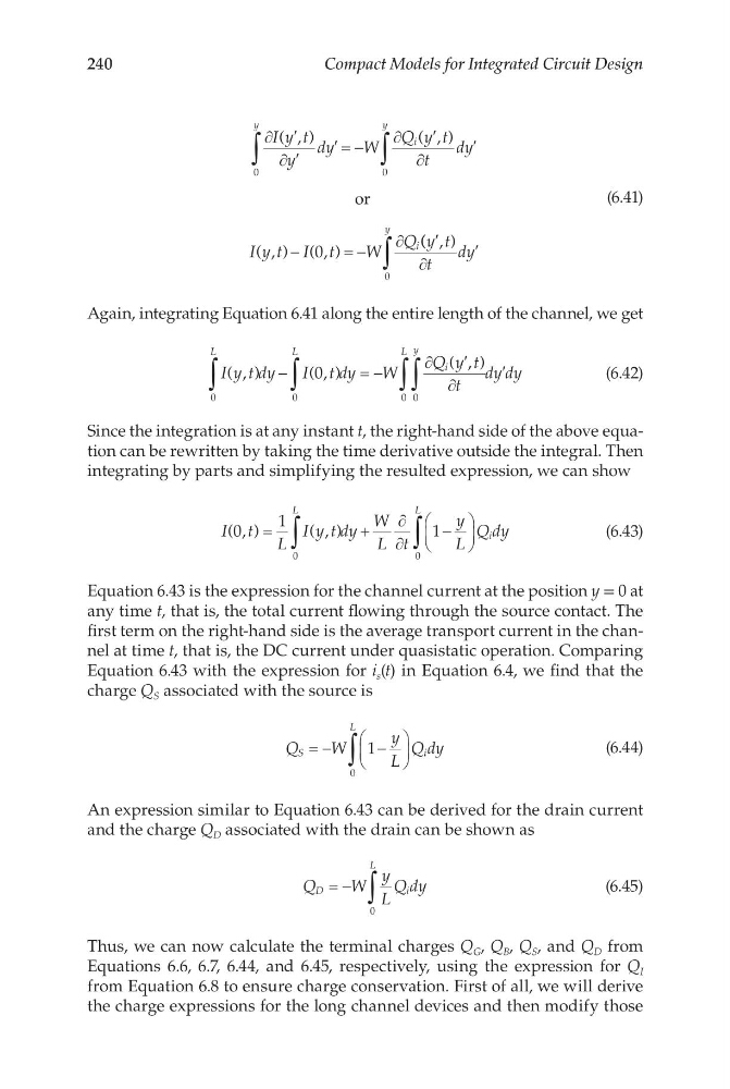
Again, integrating Equation 6.41 along the entire length of the channel, we get
I y t dy
I t dy
W
Q y t
t
dy dy
L
L
i
y
L
( , )
( , )
( , )
0
0
0
0
0
∫
∫
∫
∫
−
=−
∂
′
∂
′
(6.42)
Since the integration is at any instant t, the right-hand side of the above equation can be rewritten by taking the time derivative outside the integral. Then
integrating by parts and simplifying the resulted expression, we can show
I t L
I y t dy
W
L t
y
L
Q dy
L
i
L
( , )
( , )
0
1
1
0
0
=
+
∂
∂
−
∫
∫
(6.43)
Equation 6.43 is the expression for the channel current at the position y = 0 at
any time t, that is, the total current flowing through the source contact. The
first term on the right-hand side is the average transport current in the channel at time t, that is, the DC current under quasistatic operation. Comparing
Equation 6.43 with the expression for i s (t) in Equation 6.4, we find that the
charge Q S associated with the source is
Q
W
y
L
Q dy
S
i
L
= −
−
∫
1
0
(6.44)
An expression similar to Equation 6.43 can be derived for the drain current
and the charge Q D associated with the drain can be shown as
Q
W
y
L
Q dy
D
i
L
= −
∫
0
(6.45)
Thus, we can now calculate the terminal charges Q G , Q B , Q S , and Q D from
Equations 6.6, 6.7, 6.44, and 6.45, respectively, using the expression for Q I
from Equation 6.8 to ensure charge conservation. First of all, we will derive
the charge expressions for the long channel devices and then modify those
Compact Models for Integrated Circuit Design
∂ ′
∂ ′
′ = −
∂
′
∂
′
−
=−
∂
∫
∫
I y t
y
dy
W
Q y t
t
dy
I y t I t
W
Q
y
i
y
i
( , )
( , )
( , ) ( , )
0
0
0
or
( ( , )
′
∂
′
∫
y t
t
dy
y
0
(6.41)
Again, integrating Equation 6.41 along the entire length of the channel, we get
I y t dy
I t dy
W
Q y t
t
dy dy
L
L
i
y
L
( , )
( , )
( , )
0
0
0
0
0
∫
∫
∫
∫
−
=−
∂
′
∂
′
(6.42)
Since the integration is at any instant t, the right-hand side of the above equation can be rewritten by taking the time derivative outside the integral. Then
integrating by parts and simplifying the resulted expression, we can show
I t L
I y t dy
W
L t
y
L
Q dy
L
i
L
( , )
( , )
0
1
1
0
0
=
+
∂
∂
−
∫
∫
(6.43)
Equation 6.43 is the expression for the channel current at the position y = 0 at
any time t, that is, the total current flowing through the source contact. The
first term on the right-hand side is the average transport current in the channel at time t, that is, the DC current under quasistatic operation. Comparing
Equation 6.43 with the expression for i s (t) in Equation 6.4, we find that the
charge Q S associated with the source is
Q
W
y
L
Q dy
S
i
L
= −
−
∫
1
0
(6.44)
An expression similar to Equation 6.43 can be derived for the drain current
and the charge Q D associated with the drain can be shown as
Q
W
y
L
Q dy
D
i
L
= −
∫
0
(6.45)
Thus, we can now calculate the terminal charges Q G , Q B , Q S , and Q D from
Equations 6.6, 6.7, 6.44, and 6.45, respectively, using the expression for Q I
from Equation 6.8 to ensure charge conservation. First of all, we will derive
the charge expressions for the long channel devices and then modify those