

239
MOSFET Capacitance Models
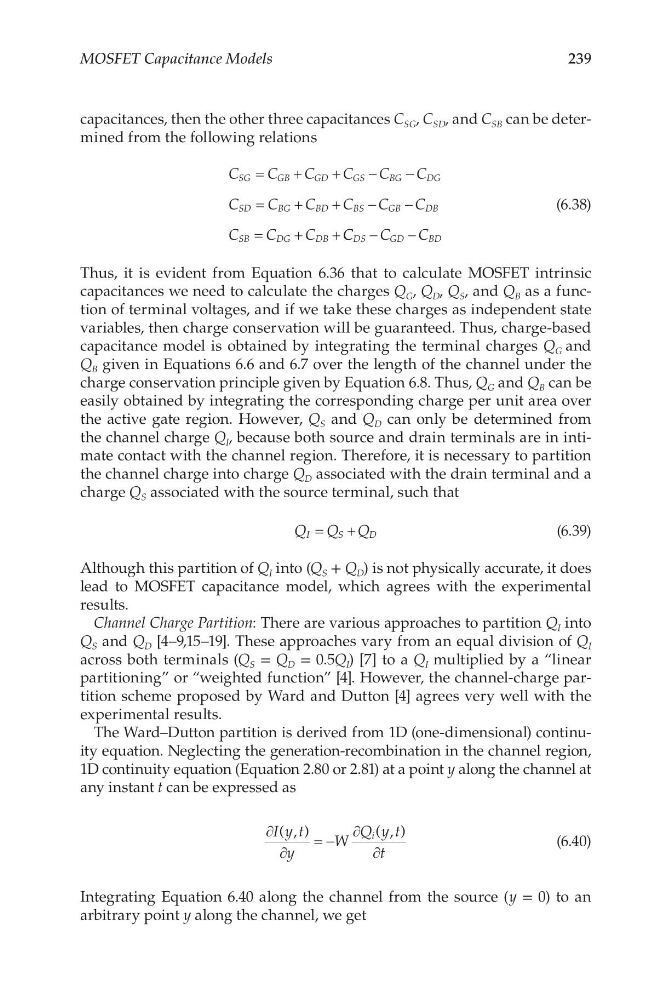
capacitances, then the other three capacitances C SG , C SD , and C SB can be determined from the following relations
C
C
C
C
C
C
C
C
C
C
C
C
C
C
C
SG
GB
GD
GS
BG
DG
SD
BG
BD
BS
GB
DB
SB
DG
DB
=
+
+
−
−
=
+
+
−
−
=
+
+ C C
C
C
DS
GD
BD
−
−
(6.38)
Thus, it is evident from Equation 6.36 that to calculate MOSFET intrinsic
capacitances we need to calculate the charges Q G , Q D , Q S , and Q B as a function of terminal voltages, and if we take these charges as independent state
variables, then charge conservation will be guaranteed. Thus, charge-based
capacitance model is obtained by integrating the terminal charges Q G and
Q B given in Equations 6.6 and 6.7 over the length of the channel under the
charge conservation principle given by Equation 6.8. Thus, Q G and Q B can be
easily obtained by integrating the corresponding charge per unit area over
the active gate region. However, Q S and Q D can only be determined from
the channel charge Q I , because both source and drain terminals are in intimate contact with the channel region. Therefore, it is necessary to partition
the channel charge into charge Q D associated with the drain terminal and a
charge Q S associated with the source terminal, such that
Q Q Q
I
S
D
=
+
(6.39)
Although this partition of Q I into (Q S + Q D ) is not physically accurate, it does
lead to MOSFET capacitance model, which agrees with the experimental
results.
Channel Charge Partition: There are various approaches to partition Q I into
Q S and Q D [4–9,15–19]. These approaches vary from an equal division of Q I
across both terminals (Q S = Q D = 0.5Q I ) [7] to a Q I multiplied by a “linear
partitioning” or “weighted function” [4]. However, the channel-charge partition scheme proposed by Ward and Dutton [4] agrees very well with the
experimental results.
The Ward–Dutton partition is derived from 1D (one-dimensional) continuity equation. Neglecting the generation-recombination in the channel region,
1D continuity equation (Equation 2.80 or 2.81) at a point y along the channel at
any instant t can be expressed as
∂
∂
= −
∂
∂
I y t
y
W
Q y t
t
i
( , )
( , )
(6.40)
Integrating Equation 6.40 along the channel from the source (y = 0) to an
arbitrary point y along the channel, we get
MOSFET Capacitance Models
capacitances, then the other three capacitances C SG , C SD , and C SB can be determined from the following relations
C
C
C
C
C
C
C
C
C
C
C
C
C
C
C
SG
GB
GD
GS
BG
DG
SD
BG
BD
BS
GB
DB
SB
DG
DB
=
+
+
−
−
=
+
+
−
−
=
+
+ C C
C
C
DS
GD
BD
−
−
(6.38)
Thus, it is evident from Equation 6.36 that to calculate MOSFET intrinsic
capacitances we need to calculate the charges Q G , Q D , Q S , and Q B as a function of terminal voltages, and if we take these charges as independent state
variables, then charge conservation will be guaranteed. Thus, charge-based
capacitance model is obtained by integrating the terminal charges Q G and
Q B given in Equations 6.6 and 6.7 over the length of the channel under the
charge conservation principle given by Equation 6.8. Thus, Q G and Q B can be
easily obtained by integrating the corresponding charge per unit area over
the active gate region. However, Q S and Q D can only be determined from
the channel charge Q I , because both source and drain terminals are in intimate contact with the channel region. Therefore, it is necessary to partition
the channel charge into charge Q D associated with the drain terminal and a
charge Q S associated with the source terminal, such that
Q Q Q
I
S
D
=
+
(6.39)
Although this partition of Q I into (Q S + Q D ) is not physically accurate, it does
lead to MOSFET capacitance model, which agrees with the experimental
results.
Channel Charge Partition: There are various approaches to partition Q I into
Q S and Q D [4–9,15–19]. These approaches vary from an equal division of Q I
across both terminals (Q S = Q D = 0.5Q I ) [7] to a Q I multiplied by a “linear
partitioning” or “weighted function” [4]. However, the channel-charge partition scheme proposed by Ward and Dutton [4] agrees very well with the
experimental results.
The Ward–Dutton partition is derived from 1D (one-dimensional) continuity equation. Neglecting the generation-recombination in the channel region,
1D continuity equation (Equation 2.80 or 2.81) at a point y along the channel at
any instant t can be expressed as
∂
∂
= −
∂
∂
I y t
y
W
Q y t
t
i
( , )
( , )
(6.40)
Integrating Equation 6.40 along the channel from the source (y = 0) to an
arbitrary point y along the channel, we get