

153
Large Geometry MOSFET Compact Models
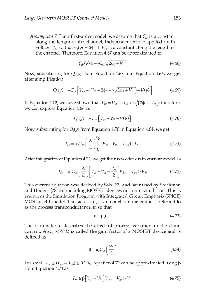
Assumption 7: For a first-order model, we assume that Q b is a constant
along the length of the channel, independent of the applied drain
voltage V ds so that f s (y) = 2f B + V sb is a constant along the length of
the channel. Therefore, Equation 4.67 can be approximated to
Q y
C
V
b
o x
B
sb
( ) ≅ −
+
γ
φ
2
(4.68)
Now, substituting for Q b (y) from Equation 4.68 into Equation 4.66, we get
after simplification
Q y
C V
V
V
V y
i
o x
g s
f b
B
B
s b
( )
( )
= −
−
+
+
+
(
) −
2
2
φ γ φ
(4.69)
In Equation 4.12, we have shown that V V
V
th
fb
B
B
sb
=
+
+
+
(
)
2
2
φ γ
φ
; therefore,
we can express Equation 4.69 as
Q y
C V V V y
i
o x
g s
t h
( )
( )
= −
−
−
(4.70)
Now, substituting for Q i (y) from Equation 4.70 in Equation 4.64, we get
I
C
W
L
V V V y dV
ds
s ox
g s
t h
Vds
=
−
−
∫
µ
( )
0
(4.71)
After integration of Equation 4.71, we get the first-order drain current model as
I
C
W
L
V V
V V
V
V
ds
s ox
g s
t h
ds
ds
gs
th
=
−
−
>
µ
2
;
(4.72)
This current equation was derived by Sah [27] and later used by Shichman
and Hodges [28] for modeling MOSFET devices in circuit simulation. This is
known as the Simulation Program with Integrated Circuit Emphasis (SPICE)
MOS Level 1 model. The factor μ s C ox is a model parameter and is referred to
as the process transconductance, κ, so that
κ µ
= s ox
C
(4.73)
The parameter κ describes the effect of process variation in the drain
current. Also, κ(W/L) is called the gain factor of a MOSFET device and is
defined as
β µ
=
s ox
C
W
L
(4.74)
For small V ds ≤ (V gs − V th ) ≤ 0.1 V, Equation 4.72 can be approximated using β
from Equation 4.74 as
I
V V V
V
V
ds
gs
th
ds
gs
th
≅
−
>
β
;
(4.75)
Large Geometry MOSFET Compact Models
Assumption 7: For a first-order model, we assume that Q b is a constant
along the length of the channel, independent of the applied drain
voltage V ds so that f s (y) = 2f B + V sb is a constant along the length of
the channel. Therefore, Equation 4.67 can be approximated to
Q y
C
V
b
o x
B
sb
( ) ≅ −
+
γ
φ
2
(4.68)
Now, substituting for Q b (y) from Equation 4.68 into Equation 4.66, we get
after simplification
Q y
C V
V
V
V y
i
o x
g s
f b
B
B
s b
( )
( )
= −
−
+
+
+
(
) −
2
2
φ γ φ
(4.69)
In Equation 4.12, we have shown that V V
V
th
fb
B
B
sb
=
+
+
+
(
)
2
2
φ γ
φ
; therefore,
we can express Equation 4.69 as
Q y
C V V V y
i
o x
g s
t h
( )
( )
= −
−
−
(4.70)
Now, substituting for Q i (y) from Equation 4.70 in Equation 4.64, we get
I
C
W
L
V V V y dV
ds
s ox
g s
t h
Vds
=
−
−
∫
µ
( )
0
(4.71)
After integration of Equation 4.71, we get the first-order drain current model as
I
C
W
L
V V
V V
V
V
ds
s ox
g s
t h
ds
ds
gs
th
=
−
−
>
µ
2
;
(4.72)
This current equation was derived by Sah [27] and later used by Shichman
and Hodges [28] for modeling MOSFET devices in circuit simulation. This is
known as the Simulation Program with Integrated Circuit Emphasis (SPICE)
MOS Level 1 model. The factor μ s C ox is a model parameter and is referred to
as the process transconductance, κ, so that
κ µ
= s ox
C
(4.73)
The parameter κ describes the effect of process variation in the drain
current. Also, κ(W/L) is called the gain factor of a MOSFET device and is
defined as
β µ
=
s ox
C
W
L
(4.74)
For small V ds ≤ (V gs − V th ) ≤ 0.1 V, Equation 4.72 can be approximated using β
from Equation 4.74 as
I
V V V
V
V
ds
gs
th
ds
gs
th
≅
−
>
β
;
(4.75)